This notebook demonstrates how to integrate third-party audio/spectrogram libraries with JupyterBioacoustic’s custom visualization interface. Each library’s spectrogram is wrapped in a function that returns the standard viz dict.
Requirements: librosa, scipy (included in demo env). opensoundscape is optional — install separately with pip install opensoundscape (requires PyTorch).
Author: Brookie Guzder-Williams (bguzder-williams@berkeley.edu)
Affiliation: The Eric and Wendy Schmidt Center for Data Science & Environment
from jupyter_bioacoustic import BioacousticAnnotator
from jupyter_bioacoustic.utils import visualizations as vis
import numpy as np
import io
import matplotlib
matplotlib.use('Agg')
import matplotlib.pyplot as plt[JBA] Debug mode enabled. Logs → /Users/brookie/code/dse/jupyter_bioacoustic/repos/jupyter_bioacoustic/demo/jba_debug.log
DATA = 'data/detections.N-dse.csv'
AUDIO = 'audio_url'
1. OpenSoundscape (optional)
OpenSoundscape provides Spectrogram and MelSpectrogram classes with built-in bandpass and trimming. It requires PyTorch, so install separately: pip install opensoundscape.
Skip this section if opensoundscape is not installed — the remaining sections work independently.
Reference: OpenSoundscape Spectrogram Tutorial
from opensoundscape import Audio, Spectrogram
from opensoundscape.spectrogram import MelSpectrogram
def oss_spectrogram(mono, sr, width):
"""OpenSoundscape linear spectrogram (matrix return).
Returns the spectrogram matrix as-is from OpenSoundscape.
OSS stores values in dB scale, so we set matrix_scale='db'
to skip the redundant dB conversion in our renderer.
"""
audio = Audio(mono, sr)
window = min(1024, len(mono) // 4)
overlap = window // 2
spec = Spectrogram.from_audio(audio, window_samples=window, overlap_samples=overlap)
return {
'matrix': spec.spectrogram,
'matrix_scale': 'db',
'freq_min': float(spec.frequencies[0]),
'freq_max': float(spec.frequencies[-1]),
'freq_scale': 'linear',
}
def oss_mel_spectrogram(mono, sr, width):
"""OpenSoundscape mel spectrogram with 400 mel bins (matrix return).
Values are already in dB from OpenSoundscape — the output should
look identical to calling melspec.plot() directly.
"""
audio = Audio(mono, sr)
melspec = MelSpectrogram.from_audio(audio, window_samples=2048, n_mels=400)
return {
'matrix': melspec.spectrogram,
'matrix_scale': 'db',
'freq_min': float(melspec.frequencies[0]),
'freq_max': float(melspec.frequencies[-1]),
'freq_scale': 'mel',
}
def oss_bandpass(mono, sr, width, f_lo=2000, f_hi=10000):
"""OpenSoundscape bandpass spectrogram (matrix return).
Uses OpenSoundscape's .bandpass() to isolate a frequency range.
"""
audio = Audio(mono, sr)
spec = Spectrogram.from_audio(audio, window_samples=1024, overlap_samples=512)
spec = spec.bandpass(f_lo, f_hi)
return {
'matrix': spec.spectrogram,
'matrix_scale': 'db',
'freq_min': float(f_lo),
'freq_max': float(f_hi),
'freq_scale': 'linear',
}BioacousticAnnotator(
data=DATA,
audio=AUDIO,
display_columns=[AUDIO],
visualizations=[
'plain',
{'fn': oss_spectrogram, 'label': 'OSS Linear'},
{'fn': oss_mel_spectrogram, 'label': 'OSS Mel (400 bins)'},
{'fn': oss_bandpass, 'label': 'OSS Bandpass (2-10 kHz)'},
],
).open()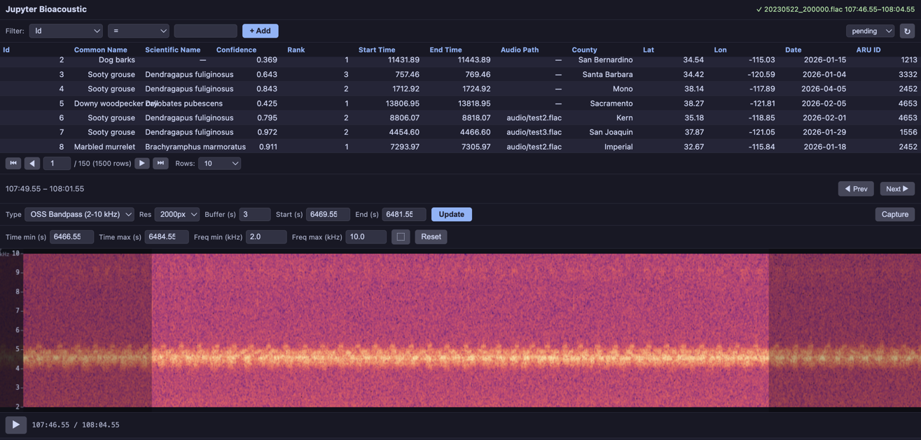
2. Librosa
Librosa is the most widely used Python audio analysis library. Here we wrap several of its spectrogram types: standard STFT, mel, and chromagram.
Reference: Librosa Spectrogram Tutorial
import librosa

def librosa_mel(mono, sr, width, n_mels=128, fmax=None):
    """Librosa mel spectrogram (matrix return).

    Uses librosa.feature.melspectrogram for mel-scale STFT with
    configurable number of mel bins.
    """
    hop = max(1, len(mono) // width) if width > 0 else 512
    S = librosa.feature.melspectrogram(
        y=mono.astype(np.float32), sr=sr,
        n_fft=2048, hop_length=hop, n_mels=n_mels, fmax=fmax,
    )
    return {
        'matrix': S,
        'freq_min': 0.0,
        'freq_max': fmax or sr / 2.0,
        'freq_scale': 'mel',
    }


def librosa_chromagram(mono, sr, width):
    """Librosa chromagram (PNG return).

    A chromagram maps audio to the 12 pitch classes (C, C#, D, ...),
    useful for harmonic analysis. Not a frequency spectrogram — the
    y-axis represents pitch class, not Hz.
    """
    hop = max(1, len(mono) // width) if width > 0 else 512
    chroma = librosa.feature.chroma_stft(
        y=mono.astype(np.float32), sr=sr,
        n_fft=2048, hop_length=hop,
    )
    fig = plt.figure(figsize=(width / 100, 5), dpi=100)
    ax = fig.add_axes([0, 0, 1, 1])
    ax.imshow(chroma, aspect='auto', origin='lower', cmap='magma', interpolation='bilinear')
    ax.set_axis_off()
    buf = io.BytesIO()
    fig.savefig(buf, format='png', dpi=100, bbox_inches='tight', pad_inches=0)
    plt.close(fig)
    return {
        'png_bytes': buf.getvalue(),
        'freq_min': 0,
        'freq_max': 12,
        'freq_scale': 'linear',
    }


def librosa_harmonic(mono, sr, width):
    """Librosa harmonic spectrogram (matrix return).

    Uses librosa's harmonic-percussive source separation (HPSS) to
    extract only the harmonic component, removing transients and noise.
    Useful for isolating tonal birdsong from background.
    """
    hop = max(1, len(mono) // width) if width > 0 else 512
    S = np.abs(librosa.stft(mono.astype(np.float32), n_fft=2048, hop_length=hop))
    S_harmonic, _ = librosa.decompose.hpss(S)
    return {
        'matrix': S_harmonic,
        'freq_min': 0.0,
        'freq_max': sr / 2.0,
        'freq_scale': 'linear',
    }
BioacousticAnnotator(
data=DATA,
audio=AUDIO,
display_columns=[AUDIO],
visualizations=[
'plain',
{'fn': librosa_mel, 'label': 'Librosa Mel (128 bins)'},
{'fn': librosa_harmonic, 'label': 'Librosa Harmonic (HPSS)'},
{'fn': librosa_chromagram, 'label': 'Librosa Chromagram'},
],
).open()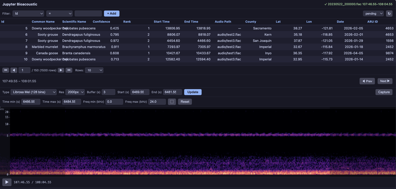
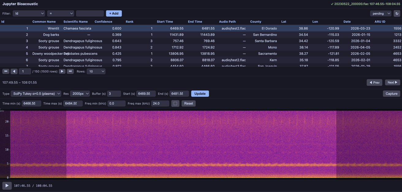
3. SciPy
SciPy’s signal module provides scipy.signal.spectrogram with configurable window functions. Different windows produce visually distinct spectrograms — here we render each with a different colormap to make the comparison obvious.
Reference: scipy
from scipy import signal as scipy_signal
from jupyter_bioacoustic.utils.visualizations import render_png


def scipy_spectrogram(mono, sr, width, window='hann', nperseg=1024, cmap='magma'):
    """SciPy spectrogram with configurable window type and colormap (PNG return).

    Uses scipy.signal.spectrogram which supports many window functions:
    'hann', 'hamming', 'blackman', 'kaiser', 'tukey', etc.
    """
    hop = max(1, len(mono) // width) if width > 0 else nperseg // 4
    noverlap = nperseg - hop
    f, t, Sxx = scipy_signal.spectrogram(
        mono, fs=sr, window=window, nperseg=nperseg,
        noverlap=max(0, noverlap), mode='magnitude',
    )
    png = render_png(Sxx, width=width, cmap=cmap)
    return {
        'png_bytes': png,
        'freq_min': float(f[0]),
        'freq_max': float(f[-1]),
        'freq_scale': 'linear',
    }


def scipy_hann(mono, sr, width):
    """SciPy Hann window — the default. Rendered with 'magma' colormap."""
    return scipy_spectrogram(mono, sr, width, window='hann', nperseg=1024, cmap='magma')


def scipy_blackman(mono, sr, width):
    """SciPy Blackman window — excellent sidelobe suppression.
    Rendered with 'inferno' colormap for visual contrast."""
    return scipy_spectrogram(mono, sr, width, window='blackman', nperseg=2048, cmap='inferno')


def scipy_kaiser(mono, sr, width):
    """SciPy Kaiser window (β=14) — very high sidelobe suppression.
    Rendered with 'viridis' colormap."""
    return scipy_spectrogram(mono, sr, width, window=('kaiser', 14), nperseg=2048, cmap='viridis')


def scipy_tukey(mono, sr, width):
    """SciPy Tukey window (α=0.5) — tapered cosine, good compromise
    between rectangular and Hann. Rendered with 'plasma' colormap."""
    return scipy_spectrogram(mono, sr, width, window=('tukey', 0.5), nperseg=1024, cmap='plasma')
BioacousticAnnotator(
data=DATA,
audio=AUDIO,
display_columns=[AUDIO],
visualizations=[
'plain',
{'fn': scipy_hann, 'label': 'SciPy Hann (magma)'},
{'fn': scipy_blackman, 'label': 'SciPy Blackman (inferno)'},
{'fn': scipy_kaiser, 'label': 'SciPy Kaiser β=14 (viridis)'},
{'fn': scipy_tukey, 'label': 'SciPy Tukey α=0.5 (plasma)'},
],
).open()