Timestep Interventions

Using single-time external data for initialization and mid-simulation events

Introduction

Many ecological simulations need external spatial data at specific moments rather than as continuously varying inputs:

Use Case Example When Applied
Initial populations Tree density from forest inventory COG Step 0 (init)
Disturbance events Fire severity from satellite imagery Specific timestep
Management actions Planting density from restoration plan Scheduled timestep

This tutorial demonstrates “flat time” external data - single-timestep spatial rasters applied at specific moments. We’ll create:

  1. Initial density data - Spatially variable tree density for initialization
  2. Fire severity data - Burn severity map applied at step 5

Prerequisites:

The Simulation

Our simulation demonstrates both patterns:

  • At init: Each patch reads initial_density to determine how many trees to create
  • At step 5: A fire event applies spatially-variable mortality based on fire_severity
Code
from pathlib import Path

SOURCE_PATH = Path("../../examples/timestep_intervention.josh")
print(SOURCE_PATH.read_text())
# Timestep intervention simulation - demonstrates single-time external data
# 
# This simulation shows two patterns for using external spatial data at
# specific timesteps:
#
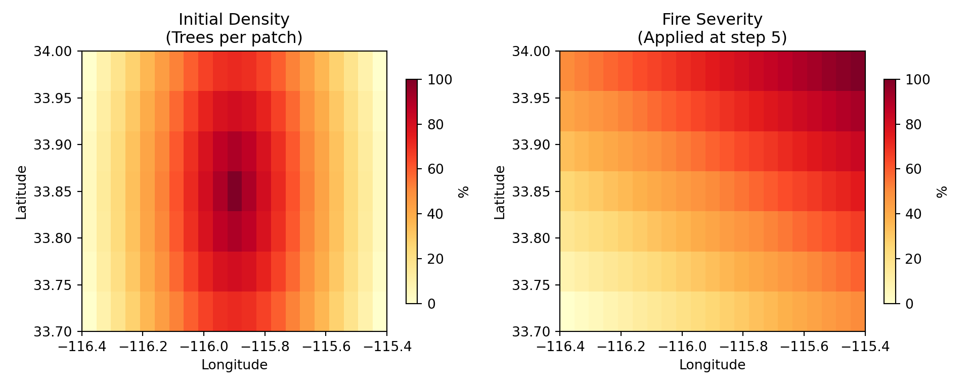
# 1. INITIAL POPULATIONS: Tree density loaded from external data at init
#    - Uses `external initial_density` in the patch's init event
#    - Creates variable number of trees per patch based on spatial data
#
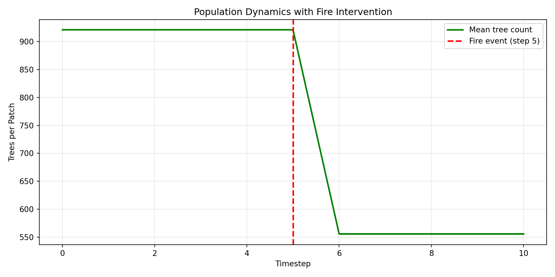
# 2. FIRE INTERVENTION: Fire severity applied at a specific timestep
#    - Uses `external fire_severity` with `meta.stepCount` conditional
#    - Applies damage only when the fire event occurs (step 5)
#
# Both patterns use "flat time" data - single-timestep spatial rasters
# that are applied at specific moments rather than varying continuously.

start simulation Main

  # Grid extent matching the external data tutorials
  grid.size = 5000 m
  grid.low = 34.0 degrees latitude, -116.4 degrees longitude
  grid.high = 33.7 degrees latitude, -115.4 degrees longitude
  grid.patch = "Default"

  # 10 timesteps to observe pre-fire growth, fire event, and recovery
  steps.low = 0 count
  steps.high = 10 count

  # Output exports to files (run_hash passed as custom-tag by joshpy)
  exportFiles.patch = "file:///tmp/timestep_intervention_{run_hash}_{replicate}.csv"

  # Fire event occurs at step 5 (configurable via meta parameter)
  fire.eventStep = 5 count

end simulation

start patch Default

  # =========================================================================
  # PATTERN 1: Initial populations from external data
  # =========================================================================
  # Read initial tree density from preprocessed spatial data at init time.
  # This value is read once at patch creation and determines tree creation.
  initial_density.init = external initial_density
  
  # Create trees based on the spatial initial density data
  # Density is 0-100%, we create trees proportional to density
  # Using a simple scaling: density/5 gives 0-20 trees per patch
  ForeverTree.init = create (initial_density / 5 percent) of ForeverTree

  # =========================================================================
  # ORGANISM REMOVAL PATTERN: Filter out dead organisms at start of step
  # =========================================================================
  # Josh does NOT have a built-in organism removal mechanism. Instead:
  # 1. Organism sets a `dead` flag when it should be removed
  # 2. Patch filters the collection at .start to exclude dead organisms
  # 
  # This is the ONLY way to reduce organism counts in Josh!
  ForeverTree.start = prior.ForeverTree[prior.ForeverTree.dead == false]

  # =========================================================================
  # PATTERN 2: Fire severity from external data at specific timestep
  # =========================================================================
  # Read fire severity from external data at INIT time (flat-time data)
  # This loads the spatial pattern once, then we use it when fire occurs
  fire_severity.init = external fire_severity
  fire_severity.step = prior.fire_severity
  
  # Detect when fire event should occur
  is_fire_step.step = meta.stepCount == meta.fire.eventStep
  
  # Calculate damage to apply (only meaningful during fire step)
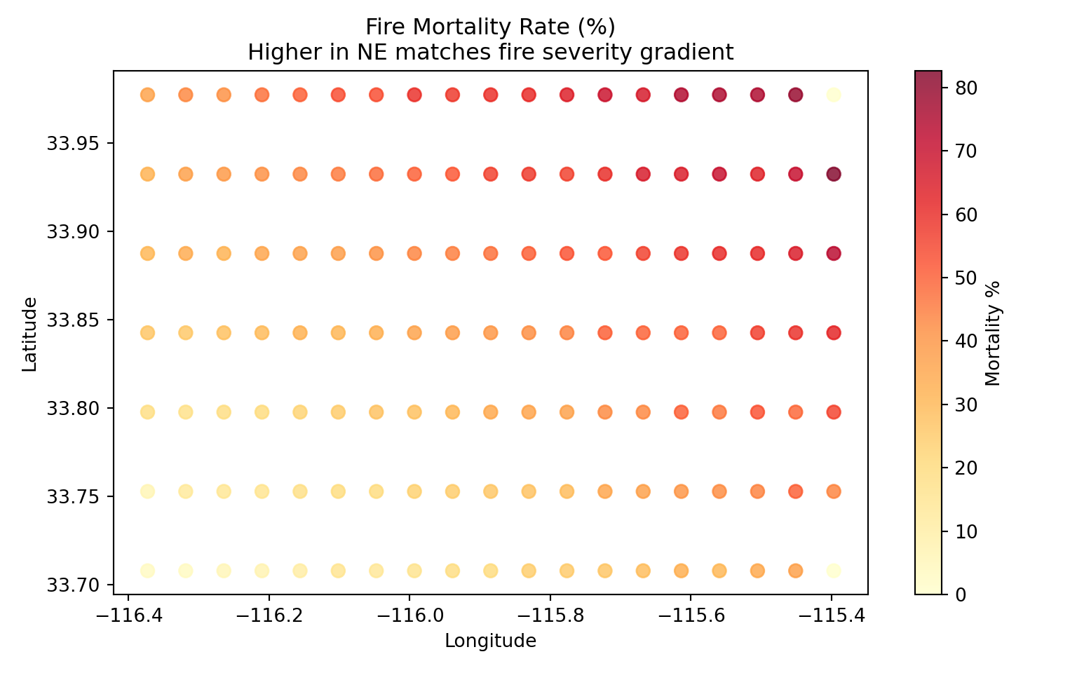
  # Severity 0-100% maps to 0-80% mortality
  fire_damage.step = map fire_severity from [0 percent, 100 percent] to [0 percent, 80 percent] linear

  # Track total tree count for exports
  tree_count.step = count(ForeverTree)
  
  # Export patch-level metrics
  export.tree_count.step = tree_count
  export.average_height.step = mean(ForeverTree.height) if tree_count > 0 count else 0 meters
  export.average_age.step = mean(ForeverTree.age) if tree_count > 0 count else 0 years
  export.fire_severity.step = fire_severity
  export.fire_damage.step = fire_damage
  export.is_fire_step.step = is_fire_step
  export.step_count.step = meta.stepCount

end patch

start organism ForeverTree

  # =========================================================================
  # Dead flag - the ONLY mechanism for organism removal in Josh
  # =========================================================================
  # The patch filters out dead organisms at .start of each step.
  # Once dead, stay dead (use prior.dead to persist the state).
  dead.init = false

  age.init = 0 years
  age.step = prior.age + 1 year

  height.init = sample uniform from 0 meters to 2 meters
  
  # Normal growth
  growth_rate.step = sample uniform from 0.5 meters to 1.5 meters
  height.step = prior.height + growth_rate

  # =========================================================================
  # Fire mortality based on patch fire severity
  # =========================================================================
  # During fire step, trees have a chance to die based on severity
  # Access patch-level fire info via 'here' keyword
  # 
  # IMPORTANT: Josh represents percentages as decimals internally (0-1 range)
  # even when specified with "percent" units. So we use count for the roll
  # to get raw 0-100 values that match fire_damage.
  survival_roll.step = sample uniform from 0 count to 100 count
  
  # Check fire step directly in organism
  is_fire_step.step = meta.stepCount == meta.fire.eventStep
  
  # Tree dies if fire is active AND survival roll is less than damage
  # Both values are now 0-100 scale
  dies_in_fire.step = is_fire_step and (survival_roll < here.fire_damage)
  
  # Mark tree as dead if it dies in fire, otherwise preserve prior state
  # This flag is read by the patch at .start to filter out dead trees
  dead.step = prior.dead or dies_in_fire

end organism

start unit year

  alias years
  alias yr
  alias yrs

end unit

Key Josh Patterns

Pattern 1: Init-time external data

# Read once at patch creation
initial_density.init = external initial_density

# Use to create variable populations (density/5 gives 0-20 trees)
ForeverTree.init = create (initial_density / 5 percent) of ForeverTree

Pattern 2: Conditional timestep events

# Read severity at init (flat-time data), persist through steps
fire_severity.init = external fire_severity
fire_severity.step = prior.fire_severity

# Detect fire step using meta.stepCount
is_fire_step.step = meta.stepCount == meta.fire.eventStep

# Apply damage conditionally - organism marks itself as dead
dies_in_fire.step = is_fire_step and (survival_roll < here.fire_damage)
dead.step = prior.dead or dies_in_fire

Pattern 3: Organism removal via patch filtering

# In the PATCH - filter out dead organisms at start of each step
ForeverTree.start = prior.ForeverTree[prior.ForeverTree.dead == false]
NoteOrganism Removal Pattern

Josh has no remove(), destroy(), or die() function. Instead, organism removal uses a two-step pattern:

  1. Organism sets a boolean flag: dead.step = prior.dead or dies_in_fire
  2. Patch filters at .start: ForeverTree.start = prior.ForeverTree[prior.ForeverTree.dead == false]

The filtering happens at .start so dead organisms are removed before the next step begins.

Step 1: Create Synthetic External Data

We create two NetCDF files with distinct spatial patterns:

File Pattern Purpose
initial_density.nc High in center, low at edges More trees in center patches
fire_severity.nc Diagonal gradient (SW to NE) Variable mortality across landscape
from pathlib import Path
import numpy as np
from scipy.io import netcdf_file

OUTPUT_DIR = Path("../../examples/external_data")
OUTPUT_DIR.mkdir(parents=True, exist_ok=True)

# Grid specification (matches timestep_intervention.josh)
LAT_MIN, LAT_MAX = 33.7, 34.0
LON_MIN, LON_MAX = -116.4, -115.4
RESOLUTION = 0.05  # Coarser resolution for faster execution

lats = np.arange(LAT_MIN, LAT_MAX + RESOLUTION, RESOLUTION)
lons = np.arange(LON_MIN, LON_MAX + RESOLUTION, RESOLUTION)
times = np.array([0.0])  # Single timestep

print(f"Grid size: {len(lats)} x {len(lons)} = {len(lats) * len(lons)} cells")
Grid size: 7 x 21 = 147 cells
def create_netcdf_flat_time(filepath, data, var_name, lats, lons, times):
    """Create a NetCDF file with a single timestep (flat time)."""
    data_3d = data[np.newaxis, :, :]  # Add time dimension
    
    with netcdf_file(str(filepath), 'w') as f:
        f.createDimension('time', len(times))
        f.createDimension('lat', len(lats))
        f.createDimension('lon', len(lons))
        
        time_var = f.createVariable('time', 'f8', ('time',))
        time_var[:] = times
        time_var.units = 'steps'
        
        lat_var = f.createVariable('lat', 'f8', ('lat',))
        lat_var[:] = lats
        lat_var.units = 'degrees_north'
        
        lon_var = f.createVariable('lon', 'f8', ('lon',))
        lon_var[:] = lons
        lon_var.units = 'degrees_east'
        
        data_var = f.createVariable(var_name, 'f4', ('time', 'lat', 'lon'))
        data_var[:] = data_3d
        data_var.units = 'percent'

# Create meshgrid for calculations
lon_grid, lat_grid = np.meshgrid(lons, lats)

# Pattern 1: Initial density - high in center, low at edges (radial)
center_lon = (LON_MIN + LON_MAX) / 2
center_lat = (LAT_MIN + LAT_MAX) / 2
max_dist = np.sqrt((LON_MAX - center_lon)**2 + (LAT_MAX - center_lat)**2)
dist_from_center = np.sqrt((lon_grid - center_lon)**2 + (lat_grid - center_lat)**2)
initial_density_data = np.maximum(0, (1 - dist_from_center / max_dist)) * 100

create_netcdf_flat_time(
    OUTPUT_DIR / "initial_density.nc",
    initial_density_data,
    "initial_density",
    lats, lons, times
)

# Pattern 2: Fire severity - diagonal gradient (SW=low, NE=high)
# Normalize both lat and lon to 0-1, then average for diagonal
lat_norm = (lat_grid - LAT_MIN) / (LAT_MAX - LAT_MIN)
lon_norm = (lon_grid - LON_MIN) / (LON_MAX - LON_MIN)
fire_severity_data = ((lat_norm + lon_norm) / 2) * 100

create_netcdf_flat_time(
    OUTPUT_DIR / "fire_severity.nc",
    fire_severity_data,
    "fire_severity",
    lats, lons, times
)

print(f"Created: initial_density.nc, fire_severity.nc")
Created: initial_density.nc, fire_severity.nc

Visualize Input Patterns

import matplotlib.pyplot as plt
from scipy.io import netcdf_file

fig, axes = plt.subplots(1, 2, figsize=(10, 4))

patterns = [
    ("initial_density.nc", "initial_density", "Initial Density\n(Trees per patch)"),
    ("fire_severity.nc", "fire_severity", "Fire Severity\n(Applied at step 5)"),
]

for ax, (filename, varname, title) in zip(axes, patterns):
    with netcdf_file(str(OUTPUT_DIR / filename), 'r') as f:
        data = f.variables[varname][0, :, :].copy()
        file_lats = f.variables['lat'][:].copy()
        file_lons = f.variables['lon'][:].copy()
    
    im = ax.imshow(data, extent=[file_lons.min(), file_lons.max(), 
                                  file_lats.min(), file_lats.max()],
                   origin='lower', cmap='YlOrRd', vmin=0, vmax=100, aspect='auto')
    ax.set_xlabel('Longitude')
    ax.set_ylabel('Latitude')
    ax.set_title(title)
    plt.colorbar(im, ax=ax, label='%', shrink=0.8)
Text(0.5, 0, 'Longitude')
Text(0, 0.5, 'Latitude')
Text(0.5, 1.0, 'Initial Density\n(Trees per patch)')
<matplotlib.colorbar.Colorbar object at 0x7fd15b6e6ba0>
Text(0.5, 0, 'Longitude')
Text(0, 0.5, 'Latitude')
Text(0.5, 1.0, 'Fire Severity\n(Applied at step 5)')
<matplotlib.colorbar.Colorbar object at 0x7fd15b528440>
plt.tight_layout()
plt.show()
Figure 1: Flat-time external data patterns for initialization and fire event

Step 2: Preprocess to JSHD Format

Convert NetCDF files to Josh’s optimized .jshd format:

from joshpy.cli import JoshCLI, NetcdfPreprocessConfig
from joshpy.jar import JarMode

cli = JoshCLI(josh_jar=JarMode.DEV)

SOURCE_PATH = Path("../../examples/timestep_intervention.josh")
DATA_DIR = Path("../../examples/external_data")

datasets = [
    ("initial_density.nc", "initial_density", "initial_density.jshd"),
    ("fire_severity.nc", "fire_severity", "fire_severity.jshd"),
]

for nc_name, var_name, jshd_name in datasets:
    print(f"Preprocessing {nc_name}...")
    
    result = cli.preprocess(NetcdfPreprocessConfig(
        script=SOURCE_PATH,
        simulation="Main",
        data_file=DATA_DIR / nc_name,
        variable=var_name,
        units="percent",
        output=DATA_DIR / jshd_name,
        x_coord="lon",
        y_coord="lat",
        time_coord="time",
    ))
    
    if result.success:
        print(f"  -> {jshd_name} created")
    else:
        raise RuntimeError(f"Preprocessing failed for {nc_name}: {result.stderr}")
Preprocessing initial_density.nc...
  -> initial_density.jshd created
Preprocessing fire_severity.nc...
  -> fire_severity.jshd created

Step 3: Configure and Run with SweepManager

We use SweepManager with fixed file_mappings (no sweep parameters - just demonstrating the timestep intervention patterns):

from pathlib import Path
from joshpy.jobs import JobConfig, SweepConfig
from joshpy.strategies import CartesianStrategy

SOURCE_PATH = Path("../../examples/timestep_intervention.josh")
TEMPLATE_PATH = Path("../../examples/templates/external_config.jshc.j2")
DATA_DIR = Path("../../examples/external_data")

config = JobConfig(
    template_path=TEMPLATE_PATH,
    source_path=SOURCE_PATH,
    simulation="Main",
    replicates=3,
    # Fixed file mappings - both files used for every run
    file_mappings={
        "initial_density": DATA_DIR / "initial_density.jshd",
        "fire_severity": DATA_DIR / "fire_severity.jshd",
    },
    # Empty sweep config - just one job with the fixed file mappings
    sweep=SweepConfig(strategy=CartesianStrategy()),
)

print(f"Replicates: {config.replicates}")
Replicates: 3
print(f"File mappings: {list(config.file_mappings.keys())}")
File mappings: ['initial_density', 'fire_severity']
from joshpy.sweep import SweepManager
from joshpy.cli import JoshCLI
from joshpy.jar import JarMode

REGISTRY_PATH = "timestep_intervention.duckdb"

manager = (
    SweepManager.builder(config)
    .with_registry(REGISTRY_PATH, experiment_name="timestep_intervention")
    .with_cli(JoshCLI(josh_jar=JarMode.DEV))
    .build()
)

print(f"Session ID: {manager.session_id}")
Session ID: 276952f2-7030-4b6c-a75f-6700783b9f1c
print(f"Total jobs: {manager.job_set.total_jobs}")
Total jobs: 1
print(f"Total replicates: {manager.job_set.total_replicates}")
Total replicates: 3
results = manager.run()
Running 1 jobs (3 total replicates)
[1/1] Running (local): {}
  [OK] Completed successfully
Completed: 1 succeeded, 0 failed
print(f"\nSimulation complete!")

Simulation complete!
print(f"Succeeded: {results.succeeded}")
Succeeded: 1
print(f"Failed: {results.failed}")
Failed: 0

# Fail the tutorial if any jobs failed - include actual error details
if results.failed > 0:
    # Extract error details from failed jobs
    errors = []
    for job, result in results:
        if not result.success:
            error_msg = result.stderr.strip() if result.stderr else "No error message"
            errors.append(f"Job {job.run_hash}: {error_msg[:500]}")
    error_detail = "\n".join(errors)
    raise RuntimeError(f"Sweep failed: {results.failed} job(s) failed\n\n{error_detail}")

Step 4: Load and Analyze Results

manager.load_results()
Loading patch results from: /tmp/timestep_intervention_{run_hash}_{replicate}.csv
  Loaded 1463 rows from timestep_intervention_f44e28d86aeb_0.csv
  Loaded 1463 rows from timestep_intervention_f44e28d86aeb_1.csv
  Loaded 1463 rows from timestep_intervention_f44e28d86aeb_2.csv

Results:
  Jobs in sweep: 1
  Jobs with results loaded: 1
  Total rows loaded: 4389
4389
summary = manager.registry.get_data_summary()
print(summary)
Registry Data Summary
========================================
Sessions: 1
Configs:  1
Runs:     1
Rows:     4,389

Variables: average_age, average_height, fire_damage, fire_severity, is_fire_step, step_count, tree_count
Entity types: patch
Parameters: (none)
Steps: 0 - 10
Replicates: 0 - 2
Spatial extent: lon [-116.37, -115.40], lat [33.71, 33.98]
print("Export variables:", manager.registry.list_export_variables())
Export variables: ['average_age', 'average_height', 'fire_damage', 'fire_severity', 'is_fire_step', 'step_count', 'tree_count']

Verify Initial Populations

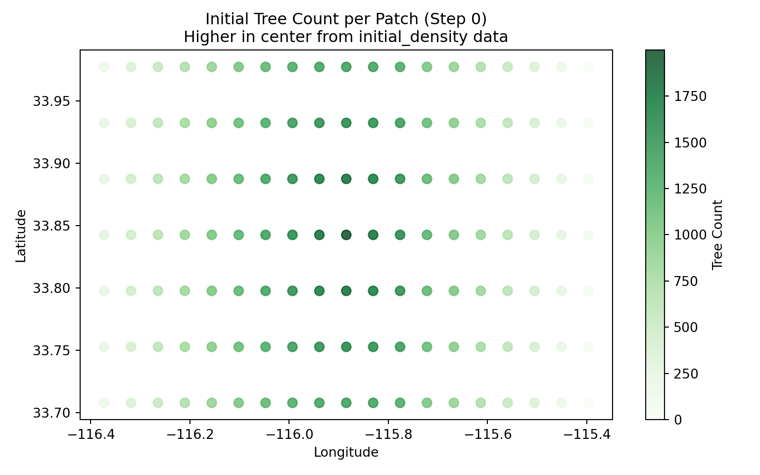
The initial density pattern should create more trees in the center:

from joshpy.cell_data import DiagnosticQueries
import matplotlib.pyplot as plt

queries = DiagnosticQueries(manager.registry)

# Get the run_hash for our single job
job = manager.job_set.jobs[0]

# Get initial state (step 0)
df_init = queries.get_spatial_snapshot(
    step=0,
    variable="tree_count",
    run_hash=job.run_hash,
    replicate=0,
)

fig, ax = plt.subplots(figsize=(8, 5))
scatter = ax.scatter(
    df_init['longitude'],
    df_init['latitude'],
    c=df_init['value'],
    cmap='Greens',
    s=50,
    alpha=0.8,
)
ax.set_xlabel('Longitude')
ax.set_ylabel('Latitude')
ax.set_title('Initial Tree Count per Patch (Step 0)\nHigher in center from initial_density data')
plt.colorbar(scatter, ax=ax, label='Tree Count')
<matplotlib.colorbar.Colorbar object at 0x7fd15066dbe0>
plt.tight_layout()
plt.show()
Figure 2: Initial tree counts reflect the radial density pattern

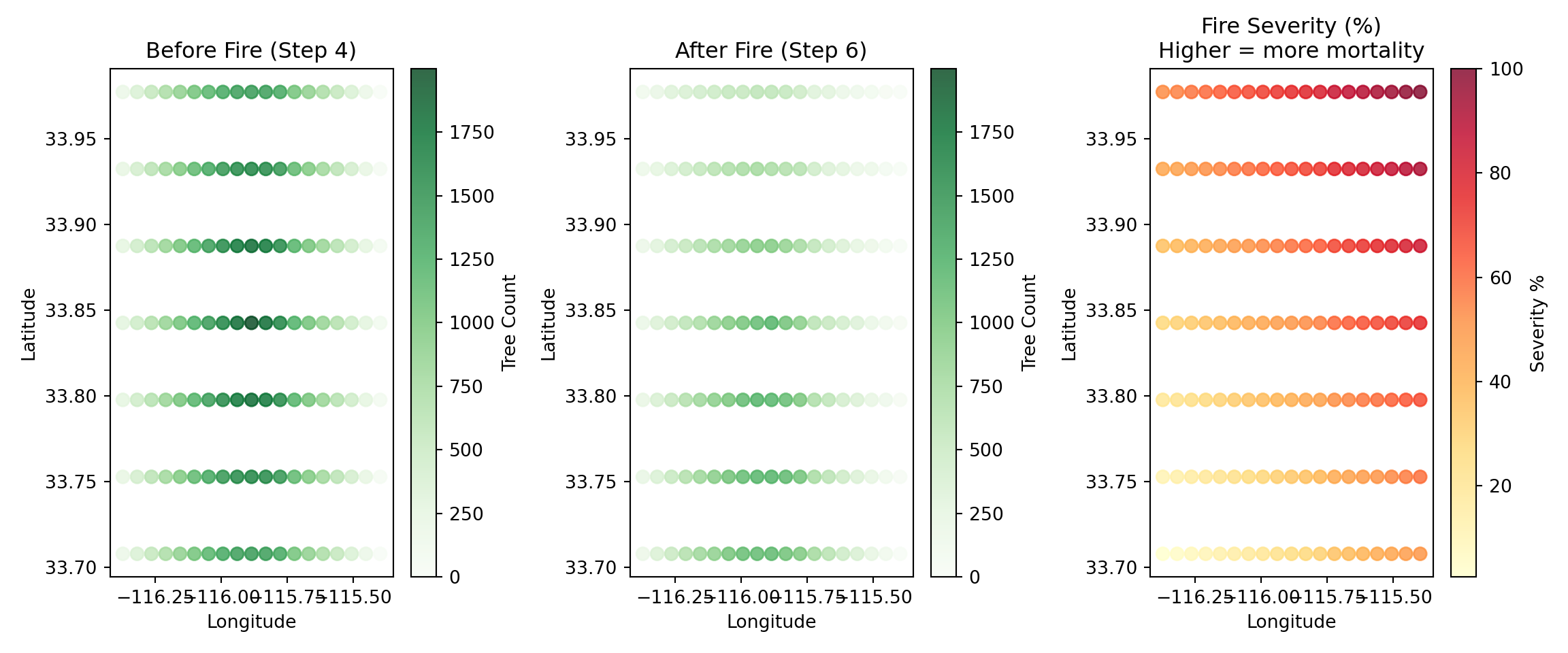
Visualize Fire Event Impact

Compare tree counts before and after the fire event at step 5:

fig, axes = plt.subplots(1, 3, figsize=(12, 5))

steps = [4, 6]
titles = ["Before Fire (Step 4)", "After Fire (Step 6)"]
max_trees = df_init['value'].max()

for ax, step, title in zip(axes[:2], steps, titles):
    df = queries.get_spatial_snapshot(
        step=step,
        variable="tree_count",
        run_hash=job.run_hash,
        replicate=0,
    )
    
    scatter = ax.scatter(
        df['longitude'],
        df['latitude'],
        c=df['value'],
        cmap='Greens',
        vmin=0,
        vmax=max_trees,
        s=50,
        alpha=0.8,
    )
    ax.set_xlabel('Longitude')
    ax.set_ylabel('Latitude')
    ax.set_title(title)
    plt.colorbar(scatter, ax=ax, label='Tree Count')
Text(0.5, 0, 'Longitude')
Text(0, 0.5, 'Latitude')
Text(0.5, 1.0, 'Before Fire (Step 4)')
<matplotlib.colorbar.Colorbar object at 0x7fd140193620>
Text(0.5, 0, 'Longitude')
Text(0, 0.5, 'Latitude')
Text(0.5, 1.0, 'After Fire (Step 6)')
<matplotlib.colorbar.Colorbar object at 0x7fd13b56c830>
# Show fire severity pattern for comparison
df_severity = queries.get_spatial_snapshot(
    step=5,
    variable="fire_severity",
    run_hash=job.run_hash,
    replicate=0,
)

scatter = axes[2].scatter(
    df_severity['longitude'],
    df_severity['latitude'],
    c=df_severity['value'],
    cmap='YlOrRd',
    s=50,
    alpha=0.8,
)
axes[2].set_xlabel('Longitude')
axes[2].set_ylabel('Latitude')
axes[2].set_title('Fire Severity (%)\nHigher = more mortality')
plt.colorbar(scatter, ax=axes[2], label='Severity %')
<matplotlib.colorbar.Colorbar object at 0x7fd13b56da90>
plt.tight_layout()
plt.show()
Figure 3: Tree counts before (step 4) and after (step 6) fire event

Time Series: Population Dynamics

# Get replicate uncertainty for tree count
df_ts = queries.get_replicate_uncertainty(
    variable="tree_count",
    run_hash=job.run_hash,
)

fig, ax = plt.subplots(figsize=(10, 5))

ax.fill_between(
    df_ts['step'],
    df_ts['mean'] - df_ts['std'],
    df_ts['mean'] + df_ts['std'],
    alpha=0.3,
    color='green'
)
ax.plot(df_ts['step'], df_ts['mean'], 'g-', linewidth=2, label='Mean tree count')
ax.axvline(5, color='red', linestyle='--', linewidth=2, label='Fire event (step 5)')

ax.set_xlabel('Timestep')
ax.set_ylabel('Trees per Patch')
ax.set_title('Population Dynamics with Fire Intervention')
ax.legend()
ax.grid(True, alpha=0.3)

plt.tight_layout()
plt.show()
Figure 4: Tree population over time with fire event at step 5

Mortality by Location

Higher fire severity in the NE should cause greater mortality there:

# Calculate mortality per patch
df_before = queries.get_spatial_snapshot(step=4, variable="tree_count", 
                                          run_hash=job.run_hash, replicate=0)
df_after = queries.get_spatial_snapshot(step=6, variable="tree_count",
                                         run_hash=job.run_hash, replicate=0)

# Merge and calculate mortality
df_before = df_before.rename(columns={'value': 'before'})
df_after = df_after.rename(columns={'value': 'after'})
df_mortality = df_before.merge(df_after[['longitude', 'latitude', 'after']], 
                                on=['longitude', 'latitude'])
df_mortality['mortality_pct'] = (
    (df_mortality['before'] - df_mortality['after']) / df_mortality['before'].clip(lower=1) * 100
)

fig, ax = plt.subplots(figsize=(8, 5))
scatter = ax.scatter(
    df_mortality['longitude'],
    df_mortality['latitude'],
    c=df_mortality['mortality_pct'],
    cmap='YlOrRd',
    s=50,
    alpha=0.8,
)
ax.set_xlabel('Longitude')
ax.set_ylabel('Latitude')
ax.set_title('Fire Mortality Rate (%)\nHigher in NE matches fire severity gradient')
plt.colorbar(scatter, ax=ax, label='Mortality %')
<matplotlib.colorbar.Colorbar object at 0x7fd0f483c830>
plt.tight_layout()
plt.show()
Figure 5: Mortality rate correlates with fire severity pattern

Key Takeaways

Flat-Time Data Patterns

Pattern Event Josh Syntax
Init-time *.init density.init = external initial_density
Conditional step *.step with guard is_fire.step = meta.stepCount == 5 count

Organism Removal Pattern

Component Role Josh Syntax
Organism flag Marks itself for removal dead.step = prior.dead or condition
Patch filter Removes flagged organisms Trees.start = prior.Trees[prior.Trees.dead == false]

The patch owns the collection and rebuilds it by filtering at each step.

When to Use Flat-Time vs Time-Varying Data

Data Type Time Dimension Use Case
Flat-time Single timestep Initial conditions, discrete events
Time-varying Multiple timesteps Climate projections, seasonal cycles

Best Practices

  1. Use meta.stepCount for timestep-conditional logic
  2. Separate concerns: Load data every step, apply conditionally
  3. Validate spatial patterns: Export and visualize intermediate values
  4. Consider stochasticity: Fire mortality uses random rolls for realistic variation
  5. Use patch-level filtering to remove organisms (not end.step or similar)
  6. Watch unit consistency: Josh stores percentages as decimals (0-1), so use count units for raw 0-100 comparisons

Summary

This tutorial demonstrated:

  1. Creating flat-time NetCDF data with single timestep for specific events
  2. Init-time patterns for spatially-variable population initialization
  3. Conditional step patterns using meta.stepCount for mid-simulation interventions
  4. Organism removal via patch-level collection filtering (the only mechanism in Josh)
  5. Visualization confirming that spatial patterns propagate correctly

The combination of spatial external data with timestep-conditional logic enables realistic scenarios like:

  • Initializing from forest inventory data
  • Applying historical fire perimeters
  • Simulating management interventions
  • Modeling disturbance-recovery dynamics

Cleanup

import os

manager.cleanup()
manager.close()

# Remove temporary registry
for f in [REGISTRY_PATH, f"{REGISTRY_PATH}.wal"]:
    if os.path.exists(f):
        os.remove(f)

Learn More