Analysis & Visualization

Explore and visualize simulation results with joshpy

Introduction

This demo focuses on exploring and visualizing simulation results after they’ve been collected. The analysis layer in joshpy is decoupled from orchestration - it only needs a RunRegistry containing data. Whether the data came from SweepManager, manual workflow, or someone else’s experiment doesn’t matter.

Prerequisites: Run either Manual Workflow or SweepManager Workflow first to generate demo_registry.duckdb.

For orchestration workflows, see:

Manual Workflow - Step-by-step control using individual components
SweepManager Workflow - Simplified workflow with SweepManager

This demo covers:

Data Discovery - What’s in the registry?
Diagnostic Plots - Quick matplotlib visualizations
Custom Queries - DiagnosticQueries for common patterns
Direct SQL - Full access to DuckDB for advanced analysis
R/ggplot2 - Publication-quality figures

Setup: Load Registry

Load the registry saved by a previous orchestration demo:

from joshpy.registry import RunRegistry

# Load registry from disk (created by manual-workflow.qmd or sweep-manager.qmd)
REGISTRY_PATH = "demo_registry.duckdb"
registry = RunRegistry(REGISTRY_PATH)

Part 1: Data Discovery

Before plotting, discover what data is available in the registry. This step is essential - column names come from your Josh exports, not from joshpy.

Discovery First

Always run list_export_variables() and list_config_parameters() before writing queries. See Best Practices: Schema & Querying for common query patterns and aggregation guidance.

Full Summary

summary = registry.get_data_summary()
print(summary)

Registry Data Summary
========================================
Sessions: 1
Configs:  10
Runs:     10
Rows:     43,890

Variables: averageAge, averageHeight
Entity types: patch
Parameters: maxGrowth
Steps: 0 - 10
Replicates: 0 - 2
Spatial extent: lon [-115.37, -114.40], lat [33.41, 33.68]

Specific Queries

# What variables were exported from the simulation?
registry.list_export_variables()

['averageAge', 'averageHeight']

# What parameters were swept?
registry.list_config_parameters()

['maxGrowth']

# What entity types are in the data?
registry.list_entity_types()

['patch']

Variable Columns

# List all variable columns in the cell_data table
registry.list_variable_columns()

['averageAge', 'averageHeight']

Part 2: Diagnostic Plots (SimulationDiagnostics)

The SimulationDiagnostics class provides quick matplotlib-based visualizations for simulation sanity checks. These are designed for rapid exploration, not publication.

from joshpy.diagnostics import SimulationDiagnostics

diag = SimulationDiagnostics(registry)

Time Series

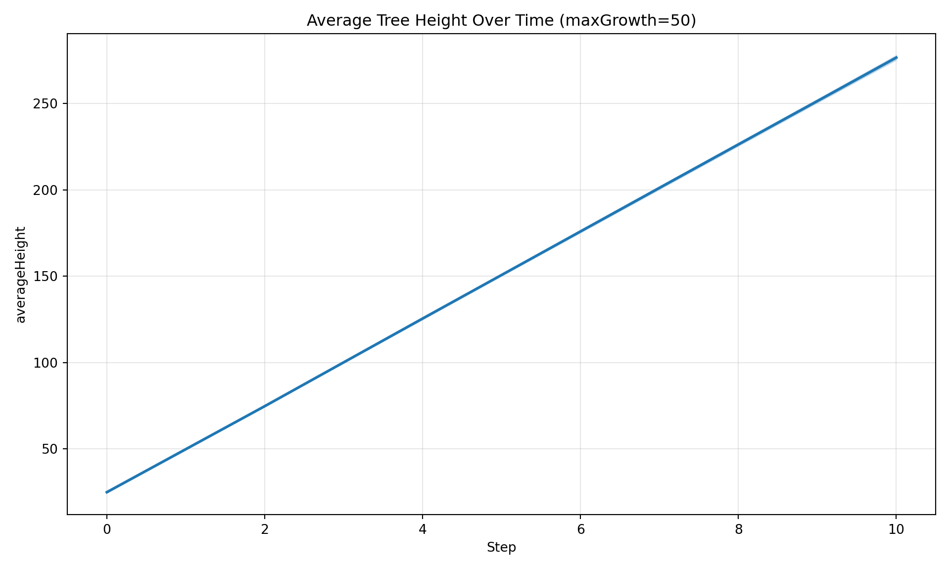
Plot how a variable evolves over simulation steps. By default, spatially aggregates across patches and shows uncertainty bands across replicates.

# Filter by parameter value
diag.plot_timeseries(
    "averageHeight",
    maxGrowth=50,
    title="Average Tree Height Over Time (maxGrowth=50)",
)

Figure 1: Tree height over time for maxGrowth=50, with replicate uncertainty.

Aggregation Options

# Sum across patches
diag.plot_timeseries("averageHeight", maxGrowth=50, aggregate="sum", title="Sum")
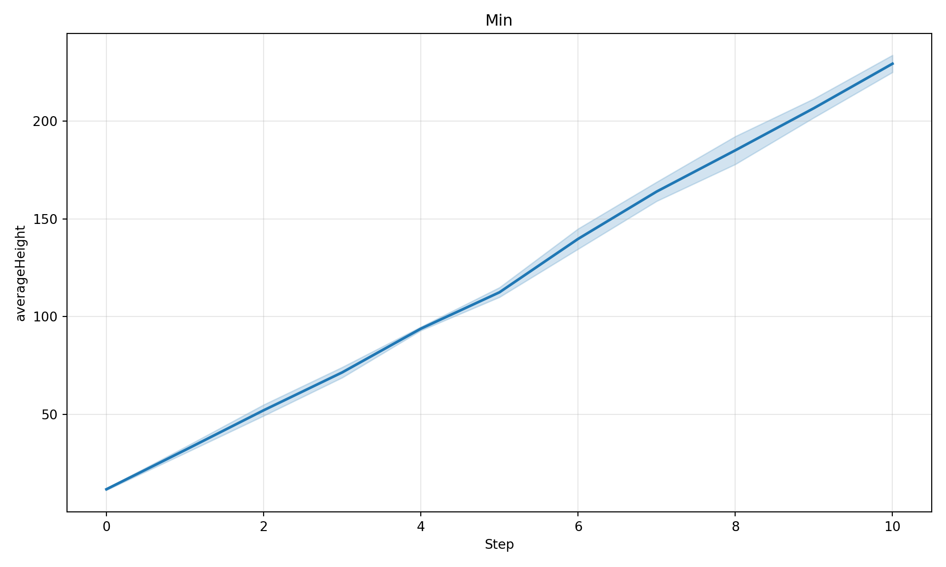
# Min across patches
diag.plot_timeseries("averageHeight", maxGrowth=50, aggregate="min", title="Min")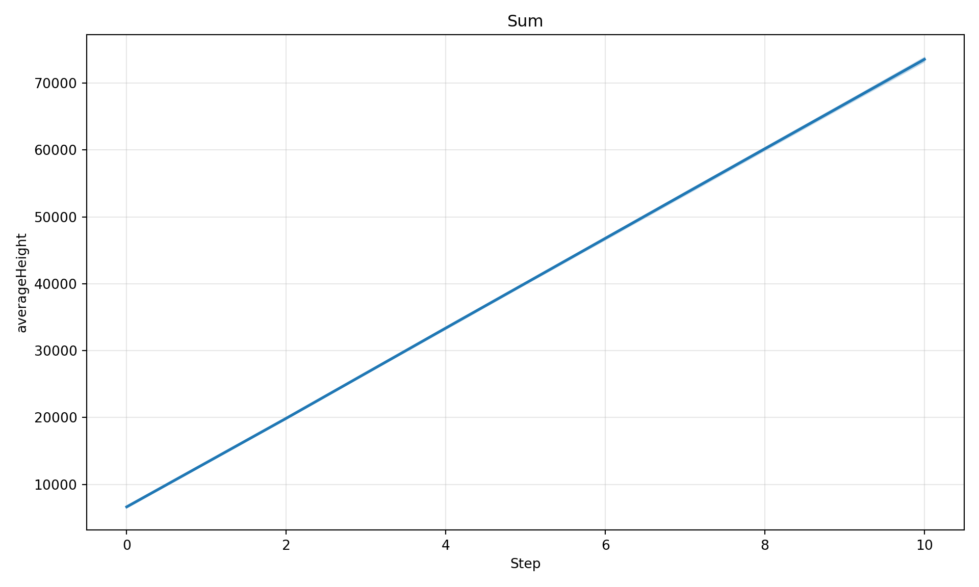

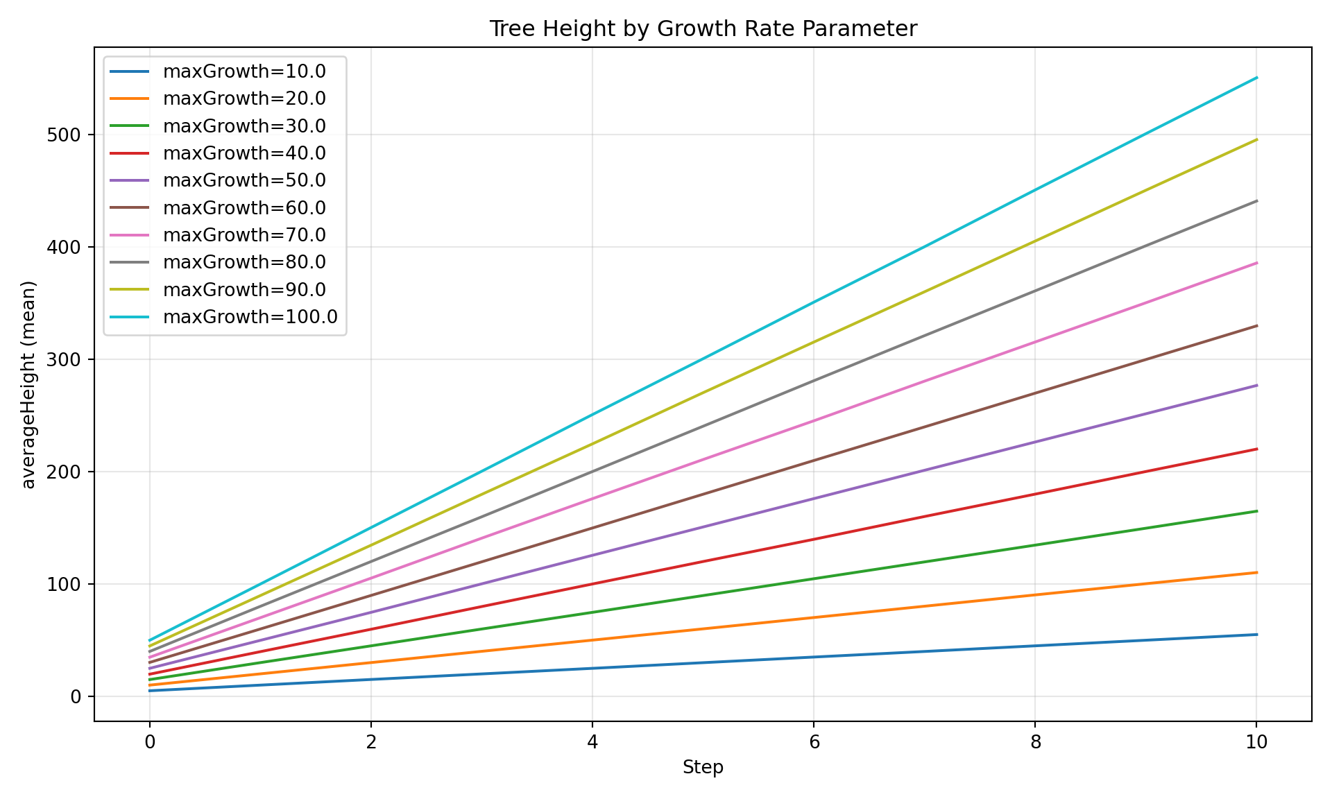
Figure 2: Different spatial aggregation methods.

Figure 3: Different spatial aggregation methods.

Parameter Comparison

Compare a variable across different parameter values - ideal for sweep results.

diag.plot_comparison(
    "averageHeight",
    group_by="maxGrowth",
    title="Tree Height by Growth Rate Parameter",
)

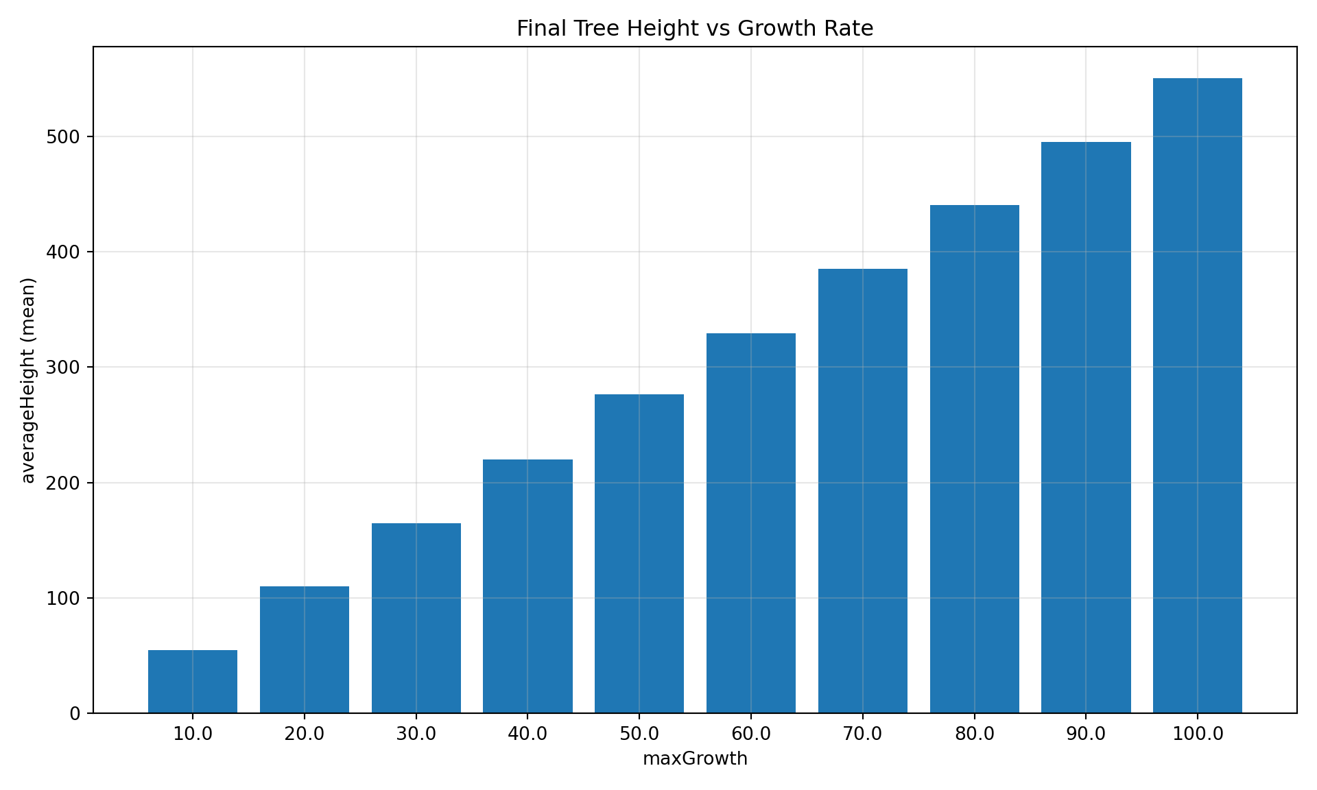
Figure 4: Tree height trajectories across all maxGrowth values.

Bar Chart at Specific Step

diag.plot_comparison(
    "averageHeight",
    group_by="maxGrowth",
    step=10,
    title="Final Tree Height vs Growth Rate",
)

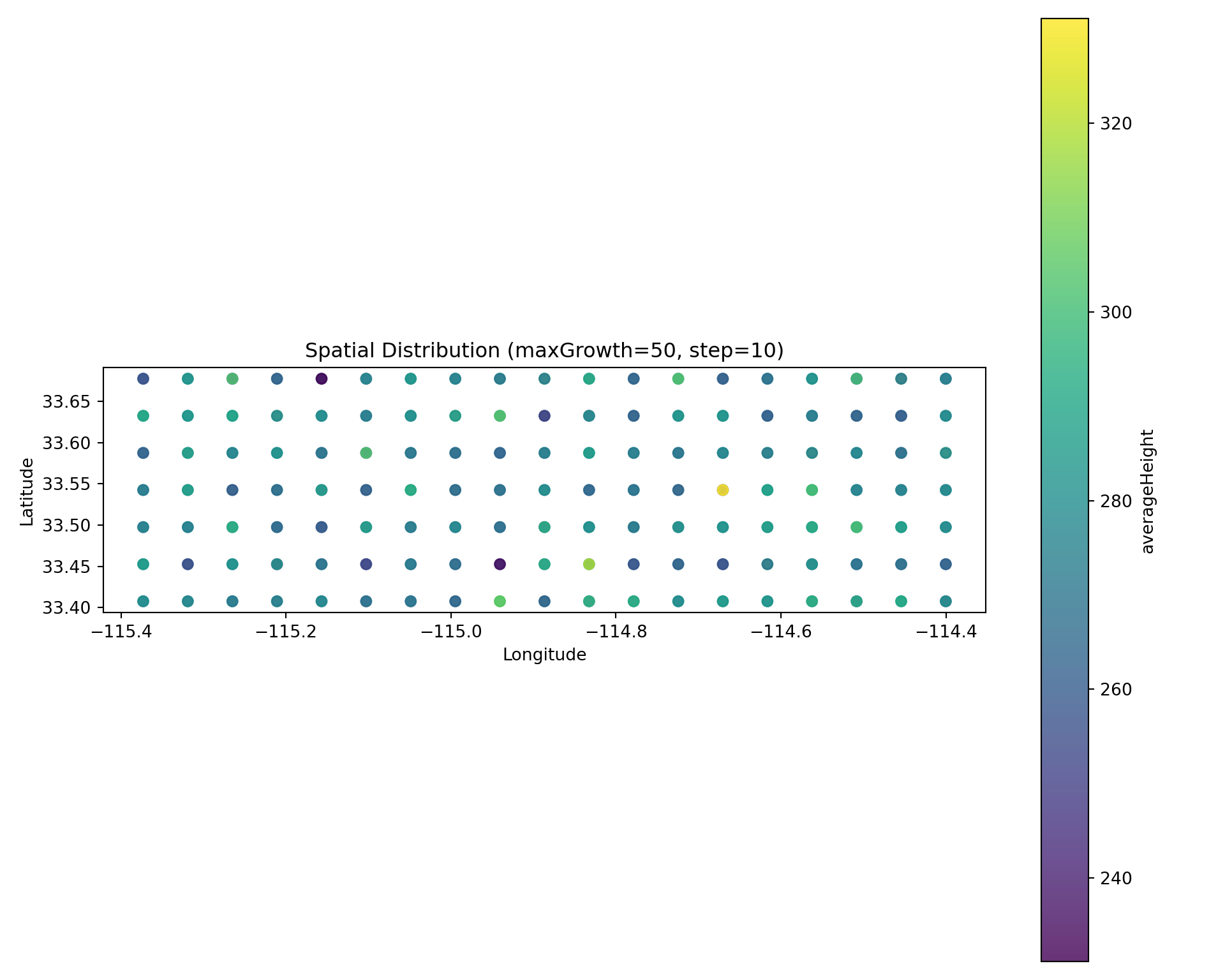
Figure 5: Final tree height (step 10) for each maxGrowth value.

Spatial Snapshot

Scatter plot colored by value at a specific timestep:

# Get a run hash for maxGrowth=50
run_hash_50 = registry.get_runs_by_parameters(maxGrowth=50)[0]["run_hash"]

diag.plot_spatial(
    "averageHeight",
    step=10,
    run_hash=run_hash_50,
    title="Spatial Distribution (maxGrowth=50, step=10)",
)

Figure 6: Spatial distribution of tree height at step 10 for maxGrowth=50.

Saving Figures

All plot methods return a matplotlib Figure that can be saved:

fig = diag.plot_comparison(
    "averageHeight",
    group_by="maxGrowth",
    show=False,  # Don't display inline
)
fig.savefig("/tmp/comparison_plot.png", dpi=150, bbox_inches="tight")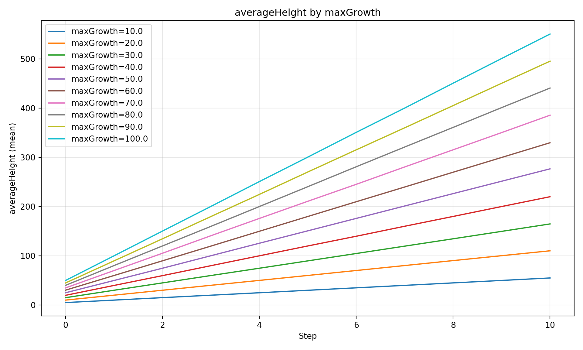

Part 3: Custom Queries (DiagnosticQueries)

For more control than SimulationDiagnostics, use DiagnosticQueries directly. These return pandas DataFrames for further processing.

from joshpy.cell_data import DiagnosticQueries

queries = DiagnosticQueries(registry)

Parameter Comparison

df = queries.get_parameter_comparison(
    variable="averageHeight",
    param_name="maxGrowth",
)
df.head(15)

	param_value	step	mean_value	std_value	n_cells
0	10.0	0	4.990825	0.914275	399
1	10.0	1	10.054546	1.244391	399
2	10.0	2	15.012953	1.548240	399
3	10.0	3	20.005701	1.847471	399
4	10.0	4	25.058594	2.014672	399
5	10.0	5	30.031544	2.194709	399
6	10.0	6	35.077375	2.397354	399
7	10.0	7	40.056394	2.636158	399
8	10.0	8	45.132441	2.798784	399
9	10.0	9	50.117931	2.962958	399
10	10.0	10	55.069338	3.150577	399
11	20.0	0	9.771987	1.809808	399
12	20.0	1	19.800545	2.610955	399
13	20.0	2	29.743859	3.267051	399
14	20.0	3	39.724835	3.775138	399

Replicate Uncertainty

Get statistics across replicates for a specific run:

df = queries.get_replicate_uncertainty(
    variable="averageHeight",
    run_hash=run_hash_50,
)
df.head(10)

	step	mean	std	ci_low	ci_high	n_replicates
0	0	25.044947	0.473936	24.508648	25.581246	3
1	1	50.248364	0.317795	49.888752	50.607976	3
2	2	75.673786	0.321899	75.309530	76.038042	3
3	3	100.530033	0.484435	99.981854	101.078212	3
4	4	125.526812	0.348489	125.132467	125.921157	3
5	5	150.787472	0.325004	150.419702	151.155242	3
6	6	175.415496	0.752038	174.564501	176.266491	3
7	7	200.361078	0.728033	199.537246	201.184910	3
8	8	225.421147	0.736903	224.587278	226.255017	3
9	9	250.298304	0.804500	249.387943	251.208665	3

Spatial Snapshot

Get all spatial data for a given timestep:

df = queries.get_spatial_snapshot(
    step=10,
    variable="averageHeight",
    run_hash=run_hash_50,
)
df.head(10)

	longitude	latitude	value
0	-114.508196	33.452687	269.959912
1	-115.210829	33.497653	287.364517
2	-115.102732	33.452687	276.273301
3	-114.778439	33.632551	272.278324
4	-114.778439	33.587585	271.014116
5	-115.318927	33.542619	276.615131
6	-114.562244	33.407720	268.089078
7	-114.508196	33.542619	276.041247
8	-114.724391	33.542619	255.923528
9	-115.210829	33.587585	309.713661

Get All Variables at Once

Retrieve all exported variables for a specific step:

df = queries.get_all_variables_at_step(
    step=10,
    run_hash=run_hash_50,
)
df.head(5)

	longitude	latitude	position_x	position_y	averageAge	averageHeight
0	-114.508196	33.452687	16.5	5.5	11.0	269.959912
1	-115.210829	33.497653	3.5	4.5	11.0	287.364517
2	-115.102732	33.452687	5.5	5.5	11.0	276.273301
3	-114.778439	33.632551	11.5	1.5	11.0	272.278324
4	-114.778439	33.587585	11.5	2.5	11.0	271.014116

Part 4: Direct SQL Queries

For full flexibility, query DuckDB directly.

Simple Aggregations

# Mean, min, max across all cells per step
result = registry.query("""
    SELECT 
        step,
        AVG(averageHeight) as mean_height,
        MIN(averageHeight) as min_height,
        MAX(averageHeight) as max_height,
        STDDEV(averageHeight) as std_height,
        COUNT(*) as n_cells
    FROM cell_data
    GROUP BY step
    ORDER BY step
""")
result.df()

	step	mean_height	min_height	max_height	std_height	n_cells
0	0	27.681788	2.821725	78.752073	15.629399	3990
1	1	55.242309	6.998114	136.550564	29.959751	3990
2	2	82.821625	10.546986	197.042799	44.345770	3990
3	3	110.122145	15.145431	246.139270	58.432869	3990
4	4	137.700887	18.950683	308.720026	72.853441	3990
5	5	165.319256	23.451497	359.712621	87.244514	3990
6	6	192.829216	27.630700	418.271207	101.571358	3990
7	7	220.272909	29.934035	479.443895	115.935966	3990
8	8	247.873201	33.037224	530.481536	130.335174	3990
9	9	275.381847	37.641517	587.912941	144.757198	3990
10	10	302.720721	42.661982	644.653712	159.088170	3990

Filtering on Variable Values

# Find cells where trees grew above a threshold
result = registry.query("""
    SELECT 
        step,
        COUNT(*) as n_cells_above_50,
        AVG(averageHeight) as mean_height_of_those
    FROM cell_data
    WHERE averageHeight > 50
    GROUP BY step
    ORDER BY step
""")
result.df()

	step	n_cells_above_50	mean_height_of_those
0	0	365	56.565190
1	1	2163	78.597847
2	2	2841	104.594483
3	3	3179	130.525999
4	4	3385	156.514972
5	5	3585	180.574037
6	6	3591	210.357199
7	7	3591	240.296967
8	8	3610	269.244289
9	9	3802	286.643922
10	10	3971	303.936274

Percentile Analysis

# Get distribution statistics per step
result = registry.query("""
    SELECT 
        step,
        APPROX_QUANTILE(averageHeight, 0.25) as p25,
        APPROX_QUANTILE(averageHeight, 0.50) as median,
        APPROX_QUANTILE(averageHeight, 0.75) as p75,
        APPROX_QUANTILE(averageHeight, 0.95) as p95
    FROM cell_data
    GROUP BY step
    ORDER BY step
""")
result.df()

	step	p25	median	p75	p95
0	0	14.603601	26.594013	39.414013	54.510150
1	1	29.880371	54.580641	79.148126	104.793557
2	2	45.072850	82.426778	119.524511	153.619784
3	3	60.105815	109.673034	159.243393	202.819378
4	4	74.816438	136.922768	198.987215	252.059392
5	5	90.171734	164.280947	239.519276	301.707617
6	6	105.229610	191.610866	280.087840	350.872525
7	7	119.829756	219.377950	320.230818	400.050208
8	8	135.308450	246.712727	359.629457	450.522048
9	9	150.404325	273.748778	400.159652	500.730780
10	10	164.853972	300.675263	440.601935	550.360618

Joining with Config Parameters

Config parameters are stored as typed columns in the config_parameters table:

# Compare results across different parameter values
result = registry.query("""
    SELECT 
        cp.maxGrowth,
        cd.step,
        AVG(cd.averageHeight) as mean_height,
        STDDEV(cd.averageHeight) as std_height
    FROM cell_data cd
    JOIN config_parameters cp ON cd.run_hash = cp.run_hash
    GROUP BY cp.maxGrowth, cd.step
    ORDER BY cp.maxGrowth, cd.step
""")
result.df().head(15)

	maxGrowth	step	mean_height	std_height
0	10.0	0	4.990825	0.914275
1	10.0	1	10.054546	1.244391
2	10.0	2	15.012953	1.548240
3	10.0	3	20.005701	1.847471
4	10.0	4	25.058594	2.014672
5	10.0	5	30.031544	2.194709
6	10.0	6	35.077375	2.397354
7	10.0	7	40.056394	2.636158
8	10.0	8	45.132441	2.798784
9	10.0	9	50.117931	2.962958
10	10.0	10	55.069338	3.150577
11	20.0	0	9.771987	1.809808
12	20.0	1	19.800545	2.610955
13	20.0	2	29.743859	3.267051
14	20.0	3	39.724835	3.775138

# Filter by parameter value (maxGrowth > 50)
result = registry.query("""
    SELECT 
        cd.step,
        AVG(cd.averageHeight) as mean_height
    FROM cell_data cd
    JOIN config_parameters cp ON cd.run_hash = cp.run_hash
    WHERE cp.maxGrowth > 50
    GROUP BY cd.step
    ORDER BY cd.step
""")
result.df()

	step	mean_height
0	0	40.272835
1	1	80.377612
2	2	120.359578
3	3	159.985498
4	4	200.152581
5	5	240.329104
6	6	280.418718
7	7	320.387910
8	8	360.484870
9	9	400.502498
10	10	440.331969

Export to File

# Export query results to CSV
registry.query("""
    SELECT step, AVG(averageHeight) as mean_height
    FROM cell_data
    GROUP BY step
    ORDER BY step
""").df().to_csv("/tmp/height_by_step.csv", index=False)

Part 5: R/ggplot2 Visualization

For publication-quality figures, there are three routes to get data from joshpy into R:

CSV Export - Simple, always works
Direct DuckDB - Custom SQL queries from R, no Python needed
py$df via reticulate - Zero-copy Python/R interop

Route 1: Export to CSV (Simple, Always Works)

# Python exports to CSV
csv_df = queries.get_parameter_comparison(
    variable="averageHeight",
    param_name="maxGrowth",
)
csv_df.to_csv("/tmp/sweep_results.csv", index=False)

# R reads CSV
df_csv <- read.csv("/tmp/sweep_results.csv")
df_csv$param_value <- as.numeric(df_csv$param_value)
head(df_csv, 5)

  param_value step mean_value std_value n_cells
1          10    0   4.990825 0.9142747     399
2          10    1  10.054546 1.2443914     399
3          10    2  15.012953 1.5482401     399
4          10    3  20.005701 1.8474706     399
5          10    4  25.058594 2.0146724     399

Pros: Always works, simple, portable
Cons: File I/O overhead, temp file management

Route 2: Direct DuckDB from R (Custom Queries)

R can query DuckDB directly with full SQL flexibility:

library(DBI)
library(duckdb)

con <- dbConnect(duckdb(), "demo_registry.duckdb", read_only = TRUE)

df_duckdb <- dbGetQuery(con, "
    SELECT 
        cp.maxGrowth as param_value,
        cd.step,
        AVG(cd.averageHeight) as mean_value,
        STDDEV(cd.averageHeight) as std_value
    FROM cell_data cd
    JOIN config_parameters cp ON cd.run_hash = cp.run_hash
    GROUP BY cp.maxGrowth, cd.step
    ORDER BY cp.maxGrowth, cd.step
")

dbDisconnect(con, shutdown = TRUE)
head(df_duckdb, 10)

   param_value step mean_value std_value
1           10    0   4.990825 0.9142747
2           10    1  10.054546 1.2443914
3           10    2  15.012953 1.5482401
4           10    3  20.005701 1.8474706
5           10    4  25.058594 2.0146724
6           10    5  30.031544 2.1947085
7           10    6  35.077375 2.3973544
8           10    7  40.056394 2.6361577
9           10    8  45.132441 2.7987839
10          10    9  50.117931 2.9629578

Pros: Full SQL flexibility, no Python needed for custom queries
Cons: Requires r-duckdb package (linux-64 only in pixi)

Route 3: `py$df` via reticulate (Zero-Copy)

In theory, you can access Python DataFrames directly via py$df:

# This should work:
# df <- reticulate::py_to_r(py$sweep_df)

We’re working on this - for now, Routes 1 and 2 are recommended.

Plotting with ggplot2

The following examples use df_duckdb from Route 2 (direct DuckDB query). We assign it to df for cleaner ggplot code:

# Use the DuckDB query result for plotting
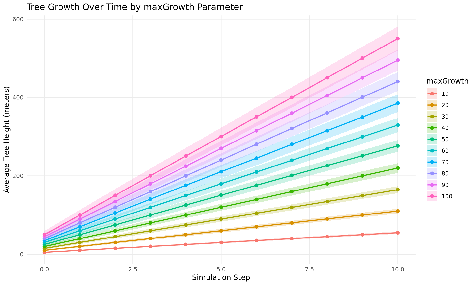
df <- df_duckdb

Time Series with Uncertainty Ribbon

ggplot(df, aes(x = step, y = mean_value, 
                     color = factor(param_value), 
                     fill = factor(param_value))) +
  geom_ribbon(aes(ymin = mean_value - std_value, 
                  ymax = mean_value + std_value), 
              alpha = 0.2, color = NA) +
  geom_line(linewidth = 0.8) +
  geom_point(size = 2) +
  labs(
    x = "Simulation Step",
    y = "Average Tree Height (meters)",
    title = "Tree Growth Over Time by maxGrowth Parameter",
    color = "maxGrowth",
    fill = "maxGrowth"
  ) +
  theme_minimal() +
  theme(
    legend.position = "right",
    panel.grid.minor = element_blank()
  )

Figure 7: Tree height trajectories with uncertainty ribbons (ggplot2).

Bar Chart with Error Bars

final_df <- df |>
  dplyr::filter(step == max(step))

ggplot(final_df, aes(x = param_value, y = mean_value)) +
  geom_col(fill = "steelblue", alpha = 0.7) +
  geom_errorbar(
    aes(ymin = mean_value - std_value, ymax = mean_value + std_value),
    width = 3,
    linewidth = 0.6
  ) +
  labs(
    x = "maxGrowth (meters/step)",
    y = "Final Average Height (meters)",
    title = "Final Tree Height vs Growth Rate"
  ) +
  theme_minimal() +
  theme(panel.grid.minor = element_blank())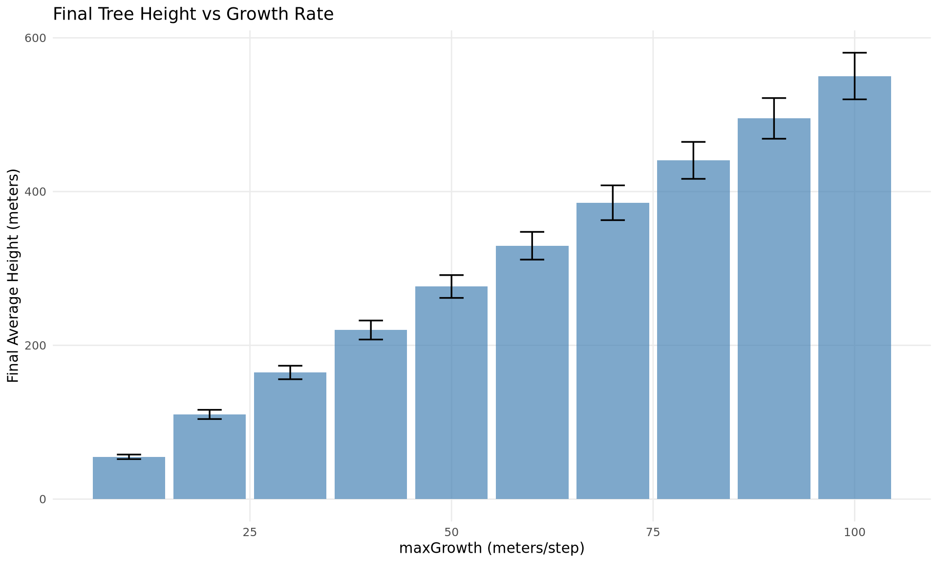

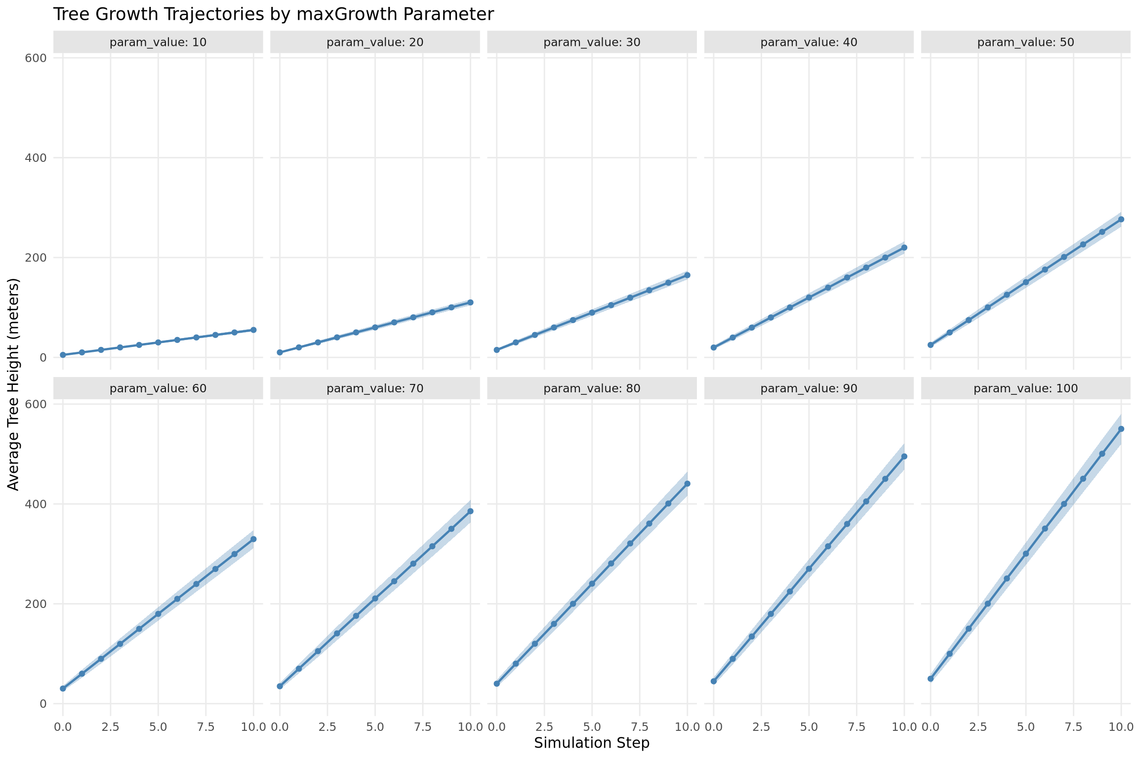
Figure 8: Final tree height vs growth rate parameter with error bars.

Faceted Plot

ggplot(df, aes(x = step, y = mean_value)) +
  geom_ribbon(aes(ymin = mean_value - std_value, 
                  ymax = mean_value + std_value), 
              alpha = 0.3, fill = "steelblue") +
  geom_line(color = "steelblue", linewidth = 0.8) +
  geom_point(color = "steelblue", size = 1.5) +
  facet_wrap(~param_value, ncol = 5, labeller = label_both) +
  labs(
    x = "Simulation Step",
    y = "Average Tree Height (meters)",
    title = "Tree Growth Trajectories by maxGrowth Parameter"
  ) +
  theme_minimal() +
  theme(
    panel.grid.minor = element_blank(),
    strip.background = element_rect(fill = "gray90", color = NA)
  )

Figure 9: Faceted time series - one panel per maxGrowth value.

Summary

This demo covered the joshpy analysis workflow:

Task	Tool	Notes
Discovery	`registry.get_data_summary()`	What’s in the registry?
Quick plots	`SimulationDiagnostics`	matplotlib-based, fast iteration
DataFrames	`DiagnosticQueries`	Returns pandas for further processing
Full SQL	`registry.query()`	Direct DuckDB access
R (CSV)	`read.csv()`	Simple, always works
R (DuckDB)	`dbConnect(duckdb(), ...)`	Custom SQL directly from R
R (reticulate)	`py$df`	Zero-copy Python/R interop

Key Points:

Analysis is decoupled from orchestration - same workflow for any data source
Export variables are typed columns in cell_data
Config parameters are typed columns in config_parameters
R can query DuckDB directly
Three routes for R: CSV export, direct DuckDB, or py$df via reticulate

Cleanup

registry.close()

Introduction

Setup: Load Registry

Part 1: Data Discovery

Full Summary

Specific Queries

Variable Columns

Part 2: Diagnostic Plots (SimulationDiagnostics)

Time Series

Aggregation Options

Parameter Comparison

Bar Chart at Specific Step

Spatial Snapshot

Saving Figures

Part 3: Custom Queries (DiagnosticQueries)

Parameter Comparison

Replicate Uncertainty

Spatial Snapshot

Get All Variables at Once

Part 4: Direct SQL Queries

Simple Aggregations

Filtering on Variable Values

Percentile Analysis

Joining with Config Parameters

Export to File

Part 5: R/ggplot2 Visualization

Route 1: Export to CSV (Simple, Always Works)

Route 2: Direct DuckDB from R (Custom Queries)

Route 3: py$df via reticulate (Zero-Copy)

Plotting with ggplot2

Time Series with Uncertainty Ribbon

Bar Chart with Error Bars

Faceted Plot

Summary

Cleanup

Route 3: `py$df` via reticulate (Zero-Copy)