Preprocessing External Data

Convert geospatial data to Josh’s optimized .jshd format

Introduction

Josh simulations can incorporate external geospatial data like climate projections, soil maps, or elevation models. Before use, this data must be preprocessed into Josh’s optimized .jshd (Josh Data) format.

Preprocessing does several things:

Spatial alignment: Resamples data to match your simulation grid
Coordinate transformation: Handles CRS conversions
Temporal alignment: Maps time steps between data and simulation
Binary optimization: Creates fast-loading binary format

Supported Input Formats

Josh supports three input formats, each with a dedicated config class:

Format	Config Class	Use Case
NetCDF	`NetcdfPreprocessConfig`	Climate projections, gridded data with time dimension
GeoTIFF/COG	`GeotiffPreprocessConfig`	Satellite imagery, elevation models, land cover maps
CSV	`CsvPreprocessConfig`	Point observations, station data

This tutorial demonstrates:

Creating synthetic test data with clear spatial patterns
Preprocessing NetCDF files using NetcdfPreprocessConfig
Preprocessing GeoTIFF files using GeotiffPreprocessConfig
Preprocessing CSV files using CsvPreprocessConfig
Verifying preprocessed data with load_jshd()

Prerequisites: joshpy installed with pip install joshpy[all]

Step 1: Create Synthetic Test Data

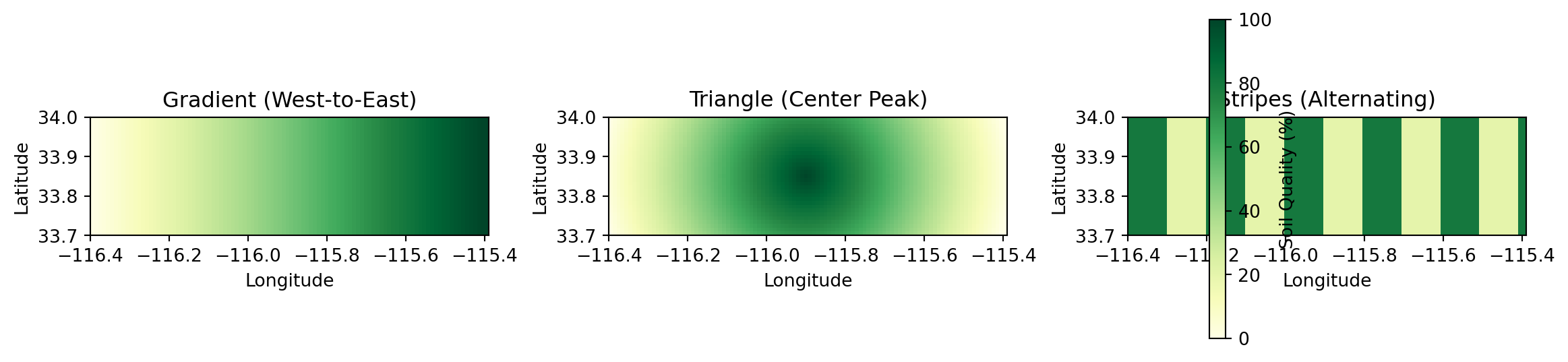
For this tutorial, we create synthetic soil quality data with three distinct spatial patterns. These patterns make it easy to verify that preprocessing works correctly and that simulations respond to external data as expected.

The Patterns

We’ll create three NetCDF files:

Pattern	Description	Expected Effect
Gradient	Soil quality increases west-to-east (0% to 100%)	Trees grow taller in the east
Triangle	Peak quality in center, decreasing to edges	Trees tallest in center
Stripes	Alternating bands of 20% and 80% quality	Bands of short and tall trees

Grid Specification

Our synthetic data matches the tutorial simulation grid:

Extent: 33.7-34.0° latitude, -116.4 to -115.4° longitude
Resolution: ~0.01° (~1km cells)
Size: Approximately 31 x 102 cells

View NetCDF Creation Code

Show NetCDF creation code

from pathlib import Path
import numpy as np
from scipy.io import netcdf_file

# Output directory
OUTPUT_DIR = Path("../../examples/external_data")
OUTPUT_DIR.mkdir(parents=True, exist_ok=True)

# Grid specification (matches external_sweep.josh)
LAT_MIN, LAT_MAX = 33.7, 34.0
LON_MIN, LON_MAX = -116.4, -115.4

# Resolution: ~0.01 degrees (~1km)
RESOLUTION = 0.01
lats = np.arange(LAT_MIN, LAT_MAX + RESOLUTION, RESOLUTION)
lons = np.arange(LON_MIN, LON_MAX + RESOLUTION, RESOLUTION)

# Single timestep - required by Josh preprocessing
times = np.array([2025.0])

print(f"Grid size: {len(lats)} x {len(lons)} = {len(lats) * len(lons)} cells")

def create_netcdf_with_time(filepath, data, lats, lons, times):
    """Create a NetCDF file with soil_quality variable and time dimension."""
    # Add time dimension to data (shape: time x lat x lon)
    data_3d = data[np.newaxis, :, :]
    
    with netcdf_file(str(filepath), 'w') as f:
        # Create dimensions
        f.createDimension('time', len(times))
        f.createDimension('lat', len(lats))
        f.createDimension('lon', len(lons))
        
        # Time variable
        time_var = f.createVariable('time', 'f8', ('time',))
        time_var[:] = times
        time_var.units = 'years'
        
        # Coordinate variables
        lat_var = f.createVariable('lat', 'f8', ('lat',))
        lat_var[:] = lats
        lat_var.units = 'degrees_north'
        
        lon_var = f.createVariable('lon', 'f8', ('lon',))
        lon_var[:] = lons
        lon_var.units = 'degrees_east'
        
        # Data variable
        soil_var = f.createVariable('soil_quality', 'f4', ('time', 'lat', 'lon'))
        soil_var[:] = data_3d
        soil_var.units = 'percent'

# Create meshgrid for calculations
lon_grid, lat_grid = np.meshgrid(lons, lats)

# Pattern 1: Gradient (west-to-east)
gradient_data = ((lon_grid - LON_MIN) / (LON_MAX - LON_MIN)) * 100
create_netcdf_with_time(OUTPUT_DIR / "soil_quality_gradient.nc", gradient_data, lats, lons, times)

# Pattern 2: Triangle (center peak)
center_lon = (LON_MIN + LON_MAX) / 2
center_lat = (LAT_MIN + LAT_MAX) / 2
max_dist = np.sqrt((LON_MAX - center_lon)**2 + (LAT_MAX - center_lat)**2)
dist_from_center = np.sqrt((lon_grid - center_lon)**2 + (lat_grid - center_lat)**2)
triangle_data = np.maximum(0, (1 - dist_from_center / max_dist)) * 100
create_netcdf_with_time(OUTPUT_DIR / "soil_quality_triangle.nc", triangle_data, lats, lons, times)

# Pattern 3: Stripes (alternating bands)
stripe_width = 0.1  # degrees longitude
stripe_index = ((lon_grid - LON_MIN) / stripe_width).astype(int)
stripes_data = np.where(stripe_index % 2 == 0, 80.0, 20.0)
create_netcdf_with_time(OUTPUT_DIR / "soil_quality_stripes.nc", stripes_data, lats, lons, times)

Created 3 NetCDF files in ../../examples/external_data
Grid size: 31 x 102 = 3162 cells

Visualize Input Patterns

import matplotlib.pyplot as plt
from scipy.io import netcdf_file
from pathlib import Path
import numpy as np

OUTPUT_DIR = Path("../../examples/external_data")

fig, axes = plt.subplots(1, 3, figsize=(12, 4))

patterns = [
    ("soil_quality_gradient.nc", "Gradient (West-to-East)"),
    ("soil_quality_triangle.nc", "Triangle (Center Peak)"),
    ("soil_quality_stripes.nc", "Stripes (Alternating)"),
]

for ax, (filename, title) in zip(axes, patterns):
    with netcdf_file(str(OUTPUT_DIR / filename), 'r') as f:
        data = f.variables['soil_quality'][0, :, :].copy()  # First timestep
        lats = f.variables['lat'][:].copy()
        lons = f.variables['lon'][:].copy()
    
    im = ax.imshow(data, extent=[lons.min(), lons.max(), lats.min(), lats.max()],
                   origin='lower', cmap='YlGn', vmin=0, vmax=100, aspect='equal')
    ax.set_xlabel('Longitude')
    ax.set_ylabel('Latitude')
    ax.set_title(title)

plt.colorbar(im, ax=axes, label='Soil Quality (%)', shrink=0.8)
plt.tight_layout()
plt.show()

Figure 1: Synthetic soil quality patterns for preprocessing

Step 2: Preprocess NetCDF with JoshCLI

The cli.preprocess() method converts geospatial data to Josh’s .jshd format. It requires a reference simulation to define the target grid.

Reference Simulation

The preprocessing command needs a Josh simulation file to know the target grid:

from pathlib import Path

SOURCE_PATH = Path("../../examples/external_sweep.josh")
print(SOURCE_PATH.read_text())

# External data sweep simulation - tree growth affected by soil quality
# Demonstrates using external geospatial data in Josh simulations
#
# The `external soil_quality` expression reads preprocessed .jshd data
# that varies spatially across the grid. Tree growth rate scales with
# soil quality, creating visible spatial patterns in the output.

start simulation Main

  # Grid extent for the tutorial area
  # Note: grid.low = northwest corner (higher lat, lower lon)
  #       grid.high = southeast corner (lower lat, higher lon)
  grid.size = 1000 m
  grid.low = 34.0 degrees latitude, -116.4 degrees longitude
  grid.high = 33.7 degrees latitude, -115.4 degrees longitude
  grid.patch = "Default"

  # 10 timesteps to observe growth patterns
  steps.low = 0 count
  steps.high = 10 count

  # Output exports to files (run_hash passed as custom-tag by joshpy)
  exportFiles.patch = "file:///tmp/external_sweep_{run_hash}_{replicate}.csv"

end simulation

start patch Default

  # Create trees in each patch
  ForeverTree.init = create 10 count of ForeverTree

  # Read soil quality from external preprocessed data
  # This value varies spatially based on the .jshd file content
  soil_quality.step = external soil_quality

  # Export patch-level averages
  export.average_height.step = mean(ForeverTree.height)
  export.average_age.step = mean(ForeverTree.age)
  export.soil_quality.step = soil_quality

end patch

start organism ForeverTree

  age.init = 0 year
  age.step = prior.age + 1 year

  height.init = 0 meters

  # Growth rate scales with soil quality from external data
  # 0% soil quality -> 0 meters max growth
  # 100% soil quality -> 10 meters max growth
  max_growth.step = map here.soil_quality from [0 percent, 100 percent] to [0 meters, 10 meters] linear

  # Actual growth is random up to max_growth
  height.step = prior.height + sample uniform from 0 meters to max_growth

end organism

start unit year

  alias years
  alias yr
  alias yrs

end unit

Preprocess Each Pattern

The output filename determines how Josh resolves external references. For example, soil_quality_gradient.jshd will be referenced as external soil_quality when passed with --data soil_quality=soil_quality_gradient.jshd.

from pathlib import Path
from joshpy.cli import JoshCLI, NetcdfPreprocessConfig
from joshpy.jar import JarMode

# Setup CLI (auto-downloads JAR if needed)
cli = JoshCLI(josh_jar=JarMode.DEV)

SOURCE_PATH = Path("../../examples/external_sweep.josh")
DATA_DIR = Path("../../examples/external_data")

# Patterns to preprocess
patterns = ["gradient", "triangle", "stripes"]

for pattern in patterns:
    nc_file = DATA_DIR / f"soil_quality_{pattern}.nc"
    jshd_file = DATA_DIR / f"soil_quality_{pattern}.jshd"

    print(f"Preprocessing {nc_file.name}...")

    result = cli.preprocess(NetcdfPreprocessConfig(
        script=SOURCE_PATH,
        simulation="Main",
        data_file=nc_file,
        variable="soil_quality",
        units="percent",
        output=jshd_file,
        x_coord="lon",
        y_coord="lat",
        time_coord="time",
        parallel=True,  # Enable parallel processing for faster preprocessing
    ))

    if result.success:
        print(f"  -> {jshd_file.name} created successfully")
    else:
        raise RuntimeError(f"Preprocessing failed for {nc_file.name}: {result.stderr}")

Preprocessing soil_quality_gradient.nc...
  -> soil_quality_gradient.jshd created successfully
Preprocessing soil_quality_triangle.nc...
  -> soil_quality_triangle.jshd created successfully
Preprocessing soil_quality_stripes.nc...
  -> soil_quality_stripes.jshd created successfully

Parallel Preprocessing

The parallel=True option enables parallel processing of grid patches, providing approximately Nx speedup on machines with N CPU cores. This is especially beneficial for large grids or when preprocessing many files. For small grids like this tutorial example, the overhead may outweigh the benefit, but for production-scale data it can significantly reduce preprocessing time.

NetcdfPreprocessConfig Options

Parameter	Description
`script`	Josh simulation file (defines target grid)
`simulation`	Name of simulation to use
`data_file`	Input NetCDF file (.nc, .nc4, .netcdf)
`variable`	NetCDF variable name to extract
`units`	Units for the data
`output`	Output `.jshd` file path
`x_coord`	Name of X/longitude dimension (default: “lon”)
`y_coord`	Name of Y/latitude dimension (default: “lat”)
`time_coord`	Name of time dimension (default: “time”)
`timestep`	Extract specific time slice (optional)
`amend`	Add to existing `.jshd` file (default: False)
`crs`	Coordinate reference system
`parallel`	Enable parallel processing (~Nx speedup on N cores)

Step 3: Verify with cli.inspect_jshd()

Use cli.inspect_jshd() to verify that preprocessing worked correctly by spot-checking values at known coordinates.

from joshpy.cli import JoshCLI, InspectJshdConfig
from joshpy.jar import JarMode
from pathlib import Path

cli = JoshCLI(josh_jar=JarMode.DEV)
DATA_DIR = Path("../../examples/external_data")

# Test coordinates (grid space, not lat/lon)
# Grid is approximately 31 x 102 cells
test_points = [
    (0, 15, "West edge"),
    (50, 15, "Center"),
    (100, 15, "East edge"),
]

print("Gradient pattern (should increase west-to-east):")
for x, y, label in test_points:
    result = cli.inspect_jshd(InspectJshdConfig(
        jshd_file=DATA_DIR / "soil_quality_gradient.jshd",
        variable="data",  # Preprocessed data stored as 'data'
        timestep=0,
        x=x,
        y=y,
    ))
    if result.success:
        value = result.stdout.strip()
        print(f"  ({x:3d}, {y:2d}) {label}: {value}")
    else:
        print(f"  ({x:3d}, {y:2d}) {label}: ERROR - {result.stderr[:80]}")

print("\nStripes pattern (should alternate 20/80):")
for x in [0, 10, 20, 30, 40]:
    result = cli.inspect_jshd(InspectJshdConfig(
        jshd_file=DATA_DIR / "soil_quality_stripes.jshd",
        variable="data",
        timestep=0,
        x=x,
        y=15,
    ))
    if result.success:
        value = result.stdout.strip()
        print(f"  x={x:3d}: {value}")

Gradient pattern (should increase west-to-east):
  (  0, 15) West edge: Value at (0, 15, 0): 1 percent
  ( 50, 15) Center: Value at (50, 15, 0): 55 percent
  (100, 15) East edge: ERROR - No value found at coordinates (100, 15) for timestep 0 in variable 'data'


Stripes pattern (should alternate 20/80):
  x=  0: Value at (0, 15, 0): 80 percent
  x= 10: Value at (10, 15, 0): 20 percent
  x= 20: Value at (20, 15, 0): 80 percent
  x= 30: Value at (30, 15, 0): 20 percent
  x= 40: Value at (40, 15, 0): 80 percent

Variable Name in JSHD Files

When inspecting .jshd files, the data is stored under the generic name data, not the original variable name from the NetCDF file. However, when Josh resolves external soil_quality, it uses the filename stem passed via --data, not the internal variable name.

Step 4: Visual Verification with plot_jshd()

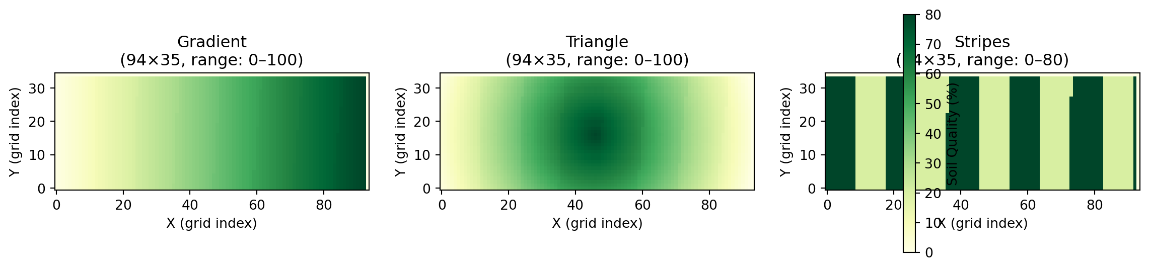
For a more comprehensive check, use load_jshd() and plot_jshd() to load the entire JSHD contents and visualize them. This is especially useful when debugging preprocessing issues or verifying spatial patterns.

import matplotlib.pyplot as plt
from pathlib import Path
from joshpy import JoshCLI, load_jshd, plot_jshd
from joshpy.jar import JarMode

cli = JoshCLI(josh_jar=JarMode.DEV)
DATA_DIR = Path("../../examples/external_data")

patterns = ["gradient", "triangle", "stripes"]

fig, axes = plt.subplots(1, 3, figsize=(12, 4))

for ax, pattern in zip(axes, patterns):
    jshd_path = DATA_DIR / f"soil_quality_{pattern}.jshd"
    
    # Load JSHD data
    data = load_jshd(cli, jshd_path)
    arr = data.to_array(timestep=0)
    
    # Plot
    im = ax.imshow(arr, origin="lower", cmap="YlGn", aspect="equal")
    ax.set_xlabel("X (grid index)")
    ax.set_ylabel("Y (grid index)")
    ax.set_title(f"{pattern.title()}\n({data.metadata.width}×{data.metadata.height}, "
                 f"range: {arr.min():.0f}–{arr.max():.0f})")

plt.colorbar(im, ax=axes, label="Soil Quality (%)", shrink=0.8)
plt.tight_layout()
plt.show()

Figure 2: Visual verification of preprocessed JSHD files showing all three spatial patterns

The visualization confirms that preprocessing preserved the spatial patterns:

Gradient: Values increase from left (low) to right (high)
Triangle: Values peak in the center and decrease toward edges
Stripes: Alternating bands of low (20%) and high (80%) values

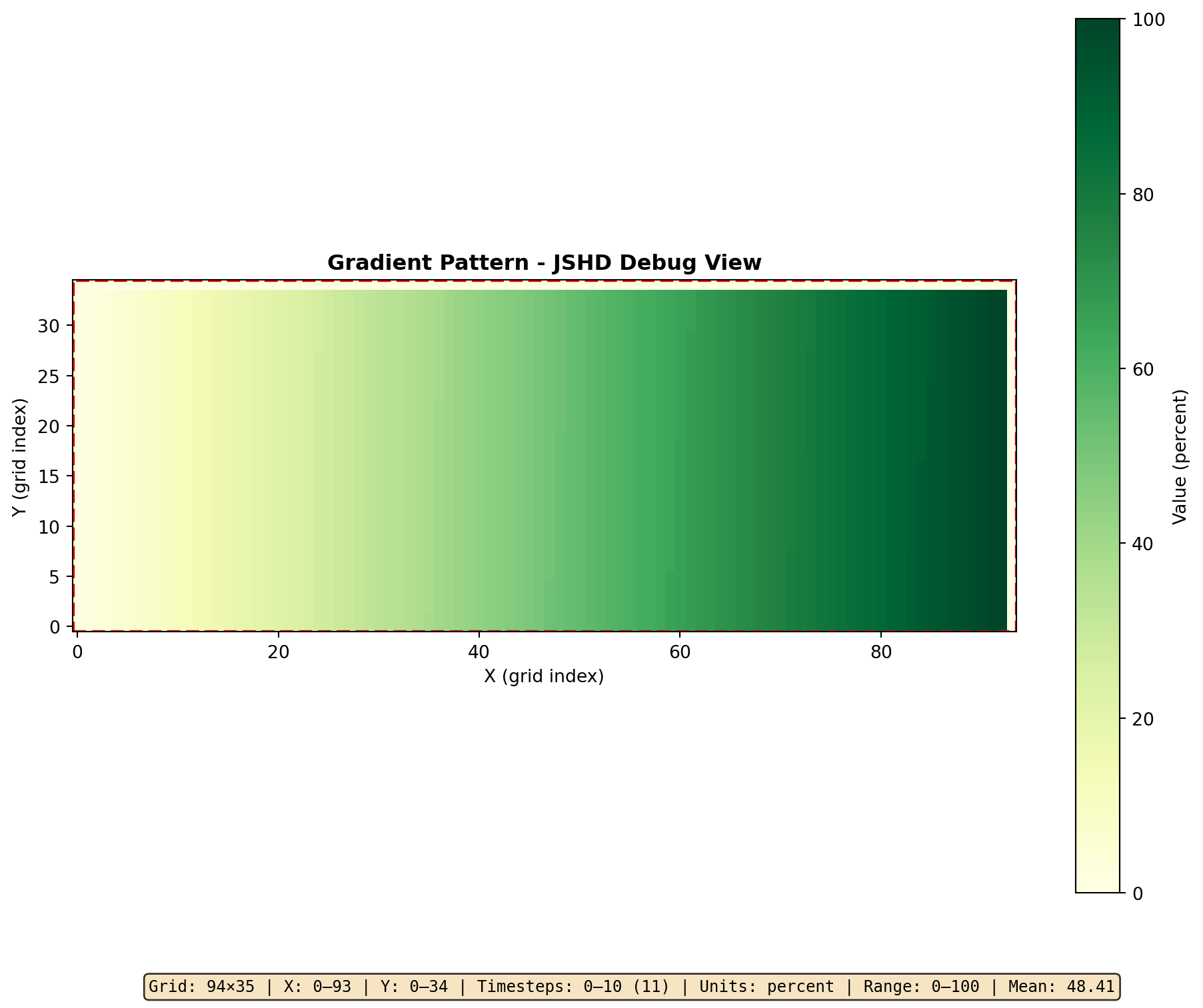
Single File Inspection

For detailed inspection of a single file, use plot_jshd() directly:

data = load_jshd(cli, DATA_DIR / "soil_quality_gradient.jshd")

# Print metadata
print(f"Grid: {data.metadata.width} × {data.metadata.height}")
print(f"Timesteps: {data.metadata.num_timesteps}")
print(f"Units: {data.metadata.units}")

# Create debug plot with full metadata
fig = plot_jshd(data, timestep=0, cmap="YlGn", title="Gradient Pattern - JSHD Debug View")

Grid: 94 × 35
Timesteps: 11
Units: percent

Figure 3: Detailed JSHD inspection with metadata

Step 5: Preprocessing GeoTIFF/COG Files

GeoTIFF and Cloud-Optimized GeoTIFF (COG) files are common for satellite imagery, elevation models, and land cover data. Use GeotiffPreprocessConfig for these files.

Required: timestep Parameter

GeoTIFF files have no time dimension, so you must specify timestep to indicate which simulation step the data maps to. For initial conditions, use timestep=0.

Create Synthetic GeoTIFF

# This example requires rasterio - shown for reference
import numpy as np
import rasterio
from rasterio.transform import from_bounds

DATA_DIR = Path("../../examples/external_data")

# Grid specification (same as NetCDF examples)
LAT_MIN, LAT_MAX = 33.7, 34.0
LON_MIN, LON_MAX = -116.4, -115.4

# Create elevation data - simple gradient from west to east
width, height = 102, 31
elevation = np.tile(np.linspace(100, 500, width), (height, 1)).astype(np.float32)

# Write GeoTIFF
transform = from_bounds(LON_MIN, LAT_MIN, LON_MAX, LAT_MAX, width, height)
with rasterio.open(
    DATA_DIR / "elevation.tif",
    'w',
    driver='GTiff',
    height=height,
    width=width,
    count=1,
    dtype=elevation.dtype,
    crs='EPSG:4326',
    transform=transform,
) as dst:
    dst.write(elevation, 1)

print(f"Created elevation.tif ({width}x{height})")

Preprocess GeoTIFF

from joshpy.cli import JoshCLI, GeotiffPreprocessConfig
from joshpy.jar import JarMode
from pathlib import Path

cli = JoshCLI(josh_jar=JarMode.DEV)
SOURCE_PATH = Path("../../examples/external_sweep.josh")
DATA_DIR = Path("../../examples/external_data")

result = cli.preprocess(GeotiffPreprocessConfig(
    script=SOURCE_PATH,
    simulation="Main",
    data_file=DATA_DIR / "elevation.tif",
    band=0,                    # Band index (0-based)
    units="meters",
    output=DATA_DIR / "elevation.jshd",
    timestep=0,                # Required: maps to simulation step 0
    crs="EPSG:4326",           # Specify if not embedded in TIF
))

if result.success:
    print("GeoTIFF preprocessed successfully!")
else:
    print(f"Error: {result.stderr}")

GeotiffPreprocessConfig Options

Parameter	Description
`script`	Josh simulation file (defines target grid)
`simulation`	Name of simulation to use
`data_file`	Input GeoTIFF file (.tif, .tiff)
`band`	Band index to extract (0-based)
`units`	Units for the data
`output`	Output `.jshd` file path
`timestep`	Required: Simulation timestep this data maps to
`amend`	Add to existing `.jshd` file (default: False)
`crs`	Coordinate reference system (if not embedded in file)
`parallel`	Enable parallel processing (~Nx speedup on N cores)

GeoTIFF Coordinates

GeoTIFF spatial coordinates are embedded in the file format itself, so x_coord and y_coord options are not needed (and will be ignored if provided).

Step 6: Preprocessing CSV Point Data

CSV files are useful for point observations like weather station data or field measurements. Use CsvPreprocessConfig for CSV files.

CSV Format Requirements

CSV files must have columns named exactly longitude and latitude. All other columns are available as variables to extract.

Create Synthetic CSV

import pandas as pd
import numpy as np
from pathlib import Path

DATA_DIR = Path("../../examples/external_data")
DATA_DIR.mkdir(parents=True, exist_ok=True)

# Create weather station data
np.random.seed(42)
n_stations = 50

# Random station locations within the grid
lons = np.random.uniform(-116.4, -115.4, n_stations)
lats = np.random.uniform(33.7, 34.0, n_stations)

# Temperature increases with latitude (north is warmer in this example)
temperature = 20 + (lats - 33.7) * 30 + np.random.normal(0, 2, n_stations)

# Precipitation decreases west to east
precipitation = 500 - (lons + 116.4) * 400 + np.random.normal(0, 20, n_stations)
precipitation = np.clip(precipitation, 50, 800)

df = pd.DataFrame({
    'longitude': lons,
    'latitude': lats,
    'temperature': temperature.round(1),
    'precipitation': precipitation.round(0),
})

csv_path = DATA_DIR / "weather_stations.csv"
df.to_csv(csv_path, index=False)

print(f"Created {csv_path.name} with {len(df)} stations")
print(df.head())

Created weather_stations.csv with 50 stations
    longitude   latitude  temperature  precipitation
0 -116.025460  33.990875         28.9          330.0
1 -115.449286  33.932540         26.4          108.0
2 -115.668006  33.981850         28.6          209.0
3 -115.801342  33.968448         24.1          250.0
4 -116.243981  33.879370         24.9          407.0

Preprocess CSV

from joshpy.cli import JoshCLI, CsvPreprocessConfig
from joshpy.jar import JarMode
from pathlib import Path

cli = JoshCLI(josh_jar=JarMode.DEV)
SOURCE_PATH = Path("../../examples/external_sweep.josh")
DATA_DIR = Path("../../examples/external_data")

# Preprocess temperature
result = cli.preprocess(CsvPreprocessConfig(
    script=SOURCE_PATH,
    simulation="Main",
    data_file=DATA_DIR / "weather_stations.csv",
    variable="temperature",    # Column name to extract
    units="celsius",
    output=DATA_DIR / "station_temperature.jshd",
    timestep=0,                # Required: maps to simulation step 0
))

if result.success:
    print("Temperature CSV preprocessed successfully!")
else:
    print(f"Error: {result.stderr}")

# Preprocess precipitation
result = cli.preprocess(CsvPreprocessConfig(
    script=SOURCE_PATH,
    simulation="Main",
    data_file=DATA_DIR / "weather_stations.csv",
    variable="precipitation",
    units="mm",
    output=DATA_DIR / "station_precipitation.jshd",
    timestep=0,
))

if result.success:
    print("Precipitation CSV preprocessed successfully!")
else:
    print(f"Error: {result.stderr}")

Temperature CSV preprocessed successfully!
Precipitation CSV preprocessed successfully!

CsvPreprocessConfig Options

Parameter	Description
`script`	Josh simulation file (defines target grid)
`simulation`	Name of simulation to use
`data_file`	Input CSV file (.csv)
`variable`	Column name to extract
`units`	Units for the data
`output`	Output `.jshd` file path
`timestep`	Required: Simulation timestep this data maps to
`amend`	Add to existing `.jshd` file (default: False)
`crs`	Coordinate reference system
`parallel`	Enable parallel processing (~Nx speedup on N cores)

CSV Performance Note

CSV preprocessing uses nearest-neighbor interpolation with a brute-force O(n) scan per grid cell. This may be slow for large CSV files (thousands of points) or large simulation grids. For better performance with large datasets, consider:

Converting CSV to GeoTIFF using tools like GDAL
Using NetCDF format which supports spatial indexing

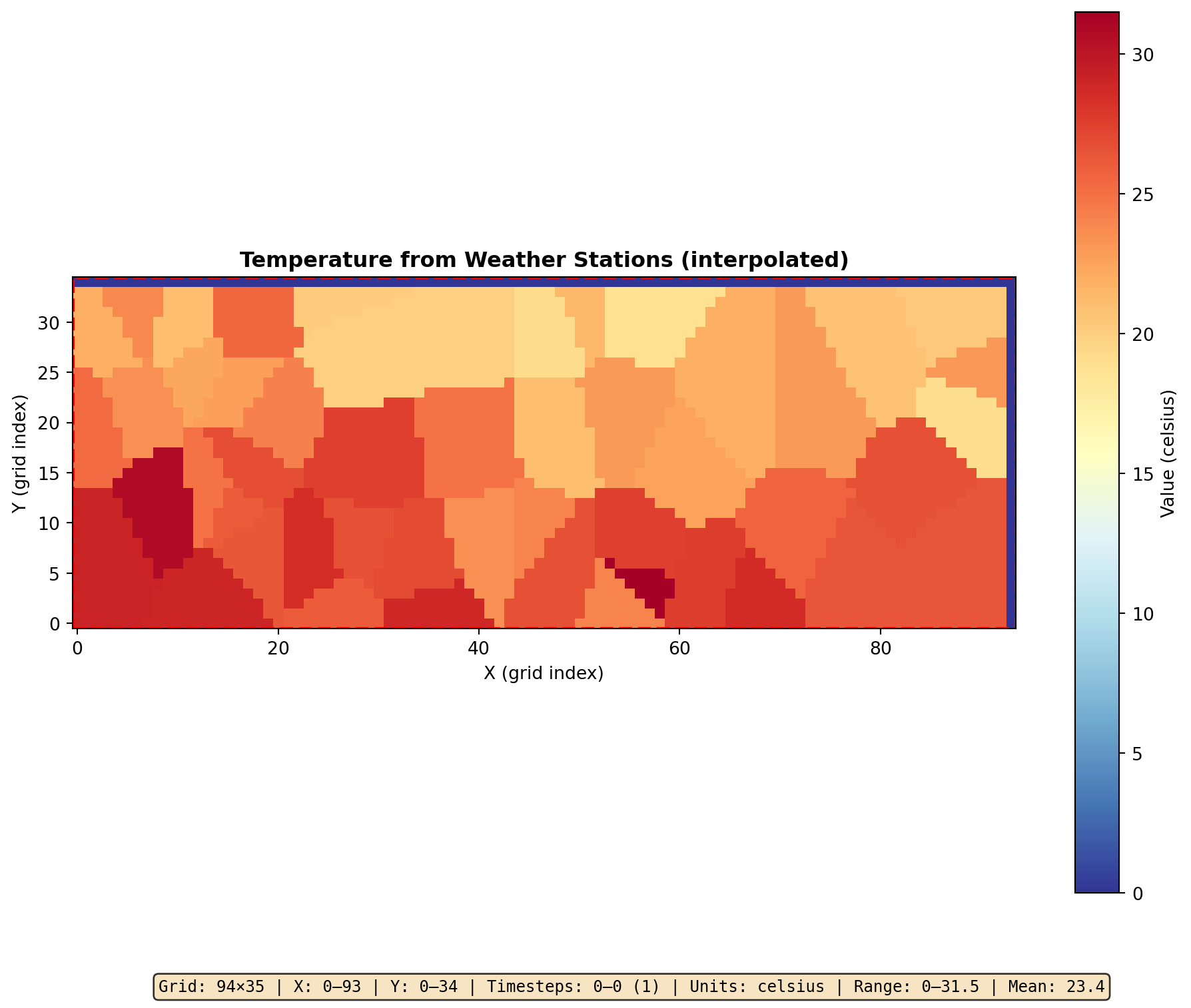
Verify CSV Preprocessing

from joshpy import load_jshd, plot_jshd

# Load and visualize
data = load_jshd(cli, DATA_DIR / "station_temperature.jshd")

print(f"Grid: {data.metadata.width} × {data.metadata.height}")
print(f"Units: {data.metadata.units}")

arr = data.to_array(timestep=0)
print(f"Value range: {arr.min():.1f} to {arr.max():.1f}")

fig = plot_jshd(data, timestep=0, cmap="RdYlBu_r", 
                title="Temperature from Weather Stations (interpolated)")

Grid: 94 × 35
Units: celsius
Value range: 0.0 to 31.5

CSV point data interpolated to simulation grid

Step 7: GridSpec-Based Preprocessing

Steps 2–6 showed the low-level cli.preprocess() API where you manage output paths and file inventories yourself. GridSpec provides a higher-level workflow: you preprocess through the grid, and it automatically registers each file and writes a grid.yaml manifest. This is the recommended approach for structured projects.

Static files (auto-registered)

When you call grid.preprocess_netcdf() without a variant argument, the output goes to output_dir/{josh_name}.jshd and the file is auto-registered in grid.files:

import tempfile
from pathlib import Path
from joshpy.grid import GridSpec
from joshpy.cli import JoshCLI
from joshpy.jar import JarMode

cli = JoshCLI(josh_jar=JarMode.DEV)
DATA_DIR = Path("../../examples/external_data")

static_dir = Path(tempfile.mkdtemp()) / "static_grid"

grid = GridSpec(
    name="tutorial_static",
    output_dir=static_dir,
    size_m=1000,
    low=(34.0, -116.4),
    high=(33.7, -115.4),
    steps=10,
)

# Preprocess — auto-registers in grid.files
result = grid.preprocess_netcdf(
    cli,
    josh_name="soil_quality",
    data_file=DATA_DIR / "soil_quality_gradient.nc",
    variable="soil_quality",
    units="percent",
    x_coord="lon",
    y_coord="lat",
    time_coord="time",
)

print(f"Success: {result.success}")
print(f"Registered files: {list(grid.files.keys())}")
print(f"Entry: {grid.files['soil_quality']}")

# Save to YAML
yaml_path = grid.save()
print(f"\n--- {yaml_path.name} ---")
print(yaml_path.read_text())

Success: True
Registered files: ['soil_quality']
Entry: {'path': 'soil_quality.jshd', 'units': 'percent'}

--- grid.yaml ---
name: tutorial_static
grid:
  size_m: 1000
  low:
  - 34.0
  - -116.4
  high:
  - 33.7
  - -115.4
  steps: 10
files:
  soil_quality:
    path: soil_quality.jshd
    units: percent

The resulting grid.yaml contains both grid geometry and the file inventory. Load it later with GridSpec.from_yaml() to get file_mappings and template_vars for JobConfig.

Variant files

When data files vary by scenario (e.g., different soil patterns or climate projections), declare variant axes in the GridSpec and preprocess each value with the variant parameter. This produces the template_path entries that power variant_sweep().

variant_dir = Path(tempfile.mkdtemp()) / "variant_grid"

grid_v = GridSpec(
    name="tutorial_variant",
    output_dir=variant_dir,
    size_m=1000,
    low=(34.0, -116.4),
    high=(33.7, -115.4),
    steps=10,
    variants={
        "pattern": {
            "values": ["gradient", "triangle", "stripes"],
            "default": "gradient",
        }
    },
    files={
        "soil_quality": {
            "template_path": "soil_quality_{pattern}.jshd",
            "units": "percent",
        }
    },
)

# Preprocess each variant value
for pattern in ["gradient", "triangle", "stripes"]:
    result = grid_v.preprocess_netcdf(
        cli,
        josh_name="soil_quality",
        variant={"pattern": pattern},
        data_file=DATA_DIR / f"soil_quality_{pattern}.nc",
        variable="soil_quality",
        units="percent",
        x_coord="lon",
        y_coord="lat",
        time_coord="time",
    )
    print(f"  {pattern}: {'OK' if result.success else 'FAIL'}")

yaml_path = grid_v.save()
print(f"\n--- {yaml_path.name} ---")
print(yaml_path.read_text())

  gradient: OK
  triangle: OK
  stripes: OK

--- grid.yaml ---
name: tutorial_variant
grid:
  size_m: 1000
  low:
  - 34.0
  - -116.4
  high:
  - 33.7
  - -115.4
  steps: 10
variants:
  pattern:
    values:
    - gradient
    - triangle
    - stripes
    default: gradient
files:
  soil_quality:
    template_path: soil_quality_{pattern}.jshd
    units: percent

Loading back

Once saved, the YAML is the single source of truth for grid geometry and data inventory:

loaded = GridSpec.from_yaml(yaml_path)

print(f"Grid: {loaded.name}")
print(f"Template vars: {loaded.template_vars}")
print(f"\nDefault file_mappings:")
for name, path in loaded.file_mappings.items():
    print(f"  {name}: {path.name}")

print(f"\nfile_mappings_for(pattern='stripes'):")
for name, path in loaded.file_mappings_for(pattern="stripes").items():
    print(f"  {name}: {path.name}")

Grid: tutorial_variant
Template vars: {'size_m': 1000, 'low_lat': 34.0, 'low_lon': -116.4, 'high_lat': 33.7, 'high_lon': -115.4, 'steps': 10}

Default file_mappings:
  soil_quality: soil_quality_gradient.jshd

file_mappings_for(pattern='stripes'):
  soil_quality: soil_quality_stripes.jshd

When to Use Which

Approach	When to use
`cli.preprocess()`	Quick one-off preprocessing, scripts, or non-grid workflows
`grid.preprocess_*()`	Structured projects where you want a `grid.yaml` manifest

Both produce identical .jshd files – the difference is whether the inventory is tracked in a YAML manifest or managed manually.

Summary

In this tutorial, we:

Created synthetic test data with clear spatial patterns using scipy.io.netcdf_file
Preprocessed NetCDF to .jshd using NetcdfPreprocessConfig
Preprocessed GeoTIFF using GeotiffPreprocessConfig (with required timestep)
Preprocessed CSV point data using CsvPreprocessConfig (with required timestep)
Verified results using cli.inspect_jshd() and plot_jshd()
Built a GridSpec manifest using grid.preprocess_netcdf() and grid.save()

The preprocessed .jshd files are now ready for use in simulations. The next tutorial, Sweeping Over External Data, demonstrates how to run parameter sweeps over multiple external data files. For the GridSpec-based variant sweep workflow, see GridSpec Variant Sweeps.

Format Comparison

Format	Config Class	`timestep`	Coordinates	Best For
NetCDF	`NetcdfPreprocessConfig`	Optional	Via `x_coord`, `y_coord`, `time_coord`	Climate data with time series
GeoTIFF	`GeotiffPreprocessConfig`	Required	Embedded in file	Raster imagery, DEMs
CSV	`CsvPreprocessConfig`	Required	Must be `longitude`, `latitude` columns	Point observations

Files Created

File	Description
`examples/external_data/soil_quality_gradient.nc`	Synthetic NetCDF - west-to-east gradient
`examples/external_data/soil_quality_triangle.nc`	Synthetic NetCDF - center peak
`examples/external_data/soil_quality_stripes.nc`	Synthetic NetCDF - alternating stripes
`examples/external_data/soil_quality_gradient.jshd`	Preprocessed - gradient pattern
`examples/external_data/soil_quality_triangle.jshd`	Preprocessed - triangle pattern
`examples/external_data/soil_quality_stripes.jshd`	Preprocessed - stripes pattern
`examples/external_data/weather_stations.csv`	Synthetic CSV - station observations
`examples/external_data/station_temperature.jshd`	Preprocessed - temperature from stations
`examples/external_data/station_precipitation.jshd`	Preprocessed - precipitation from stations

Grid Alignment & JSHD Reuse

JSHD files are tied to specific grid definitions. If you change grid.size, grid.low, or grid.high in your simulation, you must regenerate the JSHD files. See Best Practices: Preprocessing & Grid Alignment for compatibility rules and directory organization patterns.

Learn More

GridSpec Variant Sweeps - Use GridSpec variants in parameter sweeps
External Data Sweep Tutorial - Use these files in a file sweep
Project Organization - Directory layout and GridSpec conventions
Timestep Interventions - Using single-time data for events
Best Practices: Preprocessing - Grid alignment and JSHD reuse
JoshCLI Reference - CLI wrapper documentation
Josh Data Guide - Josh documentation on external data