Adaptive Parameter Optimization

Using Optuna to intelligently search parameter space

Introduction

This tutorial demonstrates adaptive parameter sweeps using Optuna’s Bayesian optimization. Unlike exhaustive grid search (CartesianStrategy), adaptive sweeps:

Learn from results: Each trial informs the next parameter selection
Focus on promising regions: Spend more trials where objectives are better
Efficient exploration: Find good parameters with fewer total trials

We’ll optimize fire damage parameters in a grass-shrub ecosystem to achieve stable vegetation dynamics (minimize coefficient of variation over time).

Prerequisites:

Familiarity with SweepManager Workflow
Install with adaptive support: pip install joshpy[adaptive]

The Model

Our grass/shrub ecosystem has balancing feedback via fire disturbance:

High vegetation cover → more frequent fires → reduced cover
Low cover → fewer fires → recovery

For a detailed walkthrough of this model, see the Grass-Shrub Fire Guide on joshsim.org.

Optimization Goal

We optimize grassDamage and shrubDamage (50-95%) to minimize the coefficient of variation (CV) of total vegetation cover over time.

The objective function:

Skips the first 50 timesteps (burn-in) to ignore transient dynamics
For each replicate, computes the spatially-averaged cover at each timestep
Computes CV = std / mean for each replicate’s time series
Returns the mean CV across all replicates

This per-replicate approach correctly detects instability even when replicates oscillate out of phase (which would be hidden by averaging across replicates first). Lower CV means more stable dynamics—the system stays near equilibrium rather than oscillating wildly.

View Configuration Template (adaptive_config.jshc.j2)

# Fire damage parameters for adaptive optimization
# Swept by Optuna to find stable vegetation dynamics

# Grass fire damage (% of cover lost per fire event)
grassDamage = {{ grassDamage }} percent

# Shrub fire damage (% of cover lost per fire event)
shrubDamage = {{ shrubDamage }} percent

View Simulation File (adaptive_fire.josh)

# Grass-shrub fire dynamics simulation for adaptive optimization demo
# Demonstrates balancing feedback for stability optimization
#
# This model creates potential for stable equilibria that depend on fire damage 
# parameters. We can optimize to find parameters that minimize population 
# variance (stability).
#
# Balancing feedback:
# - High cover -> more fires -> reduced cover
# - Low cover -> fewer fires -> growth recovers

start simulation Main

  # Small 4x4 grid for fast execution (16 patches)
  # 5km cells with bounding box sized for 4x4 layout
  grid.size = 5000 m
  grid.low = 33.8 degrees latitude, -116.0 degrees longitude
  grid.high = 33.98 degrees latitude, -115.78 degrees longitude
  grid.patch = "Default"

  # 100 steps to reach equilibrium and observe long-term stability
  steps.low = 0 count
  steps.high = 100 count

  # Output exports to files (run_hash passed as custom-tag by joshpy)
  exportFiles.patch = "file:///tmp/adaptive_fire_{run_hash}_{replicate}.csv"

  # Fire trigger parameters (fixed)
  fire.trigger.coverThreshold = 30 percent
  fire.trigger.highProb = 8 percent
  fire.trigger.typicalProb = 2 percent
  
  # Fire damage parameters (from config - swept by Optuna)
  fire.damage.grass = config adaptive_config.grassDamage
  fire.damage.shrub = config adaptive_config.shrubDamage

end simulation

start patch Default

  # Initialize vegetation cover randomly (0-30% each type)
  grassCover.init = sample uniform from 0 percent to 30 percent
  shrubCover.init = sample uniform from 0 percent to 30 percent
  
  # Total vegetation determines fire risk
  totalCover.step = prior.grassCover + prior.shrubCover
  
  # Fire probability depends on total cover
  isHighCover.step = totalCover > meta.fire.trigger.coverThreshold
  fireProbability.step = meta.fire.trigger.highProb if isHighCover else meta.fire.trigger.typicalProb
  
  # Stochastic fire occurrence
  fireRoll.step = sample uniform from 0 percent to 100 percent
  onFire.step = fireRoll < fireProbability

  # Fire damage with some variability
  damageGrass.step = sample normal with mean of meta.fire.damage.grass std of 5 percent
  damageShrub.step = sample normal with mean of meta.fire.damage.shrub std of 5 percent

  # Constant growth rates
  growthGrass.step = 4 percent
  growthShrub.step = 3 percent

  # Apply growth or fire damage
  grassCover.step = {
    const afterFire = prior.grassCover * (100 percent - damageGrass)
    const afterGrowth = prior.grassCover + growthGrass
    const newValue = afterFire if onFire else afterGrowth
    return limit newValue to [0 percent, 100 percent]
  }

  shrubCover.step = {
    const afterFire = prior.shrubCover * (100 percent - damageShrub)
    const afterGrowth = prior.shrubCover + growthShrub
    const newValue = afterFire if onFire else afterGrowth
    return limit newValue to [0 percent, 100 percent]
  }

  # Export patch-level vegetation cover
  export.grassCover.step = grassCover
  export.shrubCover.step = shrubCover
  export.totalCover.step = totalCover
  export.onFire.step = onFire

end patch

start unit year

  alias years
  alias yr

end unit

Step 1: Define the Objective Function

from joshpy.strategies import cv_objective

# Built-in objective for stability optimization
# cv_objective(variable, burn_in) returns a function that computes
# coefficient of variation (std/mean) for the given variable,
# skipping the first `burn_in` steps.
BURN_IN_STEPS = 50

stability_objective = cv_objective("totalCover", burn_in=BURN_IN_STEPS)

Custom Objectives

Objective functions have signature (registry, run_hash, job) -> float. Lower values are better (for direction="minimize"). Return float('inf') for failed/invalid runs.

Step 2: Configure with OptunaStrategy

from pathlib import Path
from joshpy.jobs import JobConfig, SweepConfig, ConfigSweepParameter
from joshpy.strategies import OptunaStrategy

SOURCE_PATH = Path("../../examples/adaptive_fire.josh")
TEMPLATE_PATH = Path("../../examples/templates/adaptive_config.jshc.j2")
DAMAGE_VALUES = list(range(50, 96, 5))  # 50, 55, ..., 95

config = JobConfig(
    template_path=TEMPLATE_PATH,
    source_path=SOURCE_PATH,
    simulation="Main",
    replicates=3,
    sweep=SweepConfig(
        config_parameters=[
            ConfigSweepParameter(name="grassDamage", values=DAMAGE_VALUES),
            ConfigSweepParameter(name="shrubDamage", values=DAMAGE_VALUES),
        ],
        strategy=OptunaStrategy(
            n_trials=30,
            direction="minimize",
            sampler="tpe",
        ),
    ),
)

Adaptive vs Cartesian Search

CartesianStrategy	OptunaStrategy
All 100 combinations	30 intelligently-chosen trials
No learning	Each trial informs the next
Exhaustive	Efficient for large spaces

Step 3: Run the Sweep

from joshpy.sweep import SweepManager
from joshpy.cli import JoshCLI
from joshpy.jar import JarMode

REGISTRY_PATH = "adaptive_demo.duckdb"

manager = (
    SweepManager.builder(config)
    .with_registry(REGISTRY_PATH, experiment_name="fire_stability")
    .with_cli(JoshCLI(josh_jar=JarMode.DEV))
    .build()
)

result = manager.run(objective=stability_objective)

[I 2026-03-27 21:40:55,668] A new study created in memory with name: no-name-de816683-8d09-43d6-8b27-9239092d3bcd
Running adaptive sweep with 30 trials
  Direction: minimize
  Sampler: tpe
[1/30] Params: {'grassDamage': 95, 'shrubDamage': 75}
  [OK] metric=0.0969 (rows=7575)
[2/30] Params: {'grassDamage': 75, 'shrubDamage': 65}
  [OK] metric=0.0952 (rows=7575)
[3/30] Params: {'grassDamage': 60, 'shrubDamage': 50}
  [OK] metric=0.0821 (rows=7575)
[4/30] Params: {'grassDamage': 50, 'shrubDamage': 90}
  [OK] metric=0.0860 (rows=7575)
[5/30] Params: {'grassDamage': 65, 'shrubDamage': 95}
  [OK] metric=0.1030 (rows=7575)
[6/30] Params: {'grassDamage': 50, 'shrubDamage': 85}
  [OK] metric=0.0701 (rows=7575)
[7/30] Params: {'grassDamage': 90, 'shrubDamage': 60}
  [OK] metric=0.0772 (rows=7575)
[8/30] Params: {'grassDamage': 90, 'shrubDamage': 65}
  [OK] metric=0.1182 (rows=7575)
[9/30] Params: {'grassDamage': 95, 'shrubDamage': 90}
  [OK] metric=0.1206 (rows=7575)
[10/30] Params: {'grassDamage': 75, 'shrubDamage': 75}
  [OK] metric=0.1238 (rows=7575)
[11/30] Params: {'grassDamage': 50, 'shrubDamage': 85}
  [OK] metric=0.0641 (rows=7575)
[12/30] Params: {'grassDamage': 50, 'shrubDamage': 85}
  [OK] metric=0.0502 (rows=7575)
[13/30] Params: {'grassDamage': 50, 'shrubDamage': 85}
  [OK] metric=0.0457 (rows=7575)
[14/30] Params: {'grassDamage': 85, 'shrubDamage': 85}
  [OK] metric=0.1139 (rows=7575)
[15/30] Params: {'grassDamage': 70, 'shrubDamage': 80}
  [OK] metric=0.1087 (rows=7575)
[16/30] Params: {'grassDamage': 55, 'shrubDamage': 55}
  [OK] metric=0.0698 (rows=7575)
[17/30] Params: {'grassDamage': 80, 'shrubDamage': 70}
  [OK] metric=0.1218 (rows=7575)
[18/30] Params: {'grassDamage': 50, 'shrubDamage': 85}
  [OK] metric=0.0390 (rows=7575)
[19/30] Params: {'grassDamage': 50, 'shrubDamage': 85}
  [OK] metric=0.0375 (rows=7575)
[20/30] Params: {'grassDamage': 70, 'shrubDamage': 95}
  [OK] metric=0.1118 (rows=7575)
[21/30] Params: {'grassDamage': 55, 'shrubDamage': 55}
  [OK] metric=0.0396 (rows=7575)
[22/30] Params: {'grassDamage': 55, 'shrubDamage': 55}
  [OK] metric=0.0335 (rows=7575)
[23/30] Params: {'grassDamage': 55, 'shrubDamage': 55}
  [OK] metric=0.0325 (rows=7575)
[24/30] Params: {'grassDamage': 55, 'shrubDamage': 55}
  [OK] metric=0.0316 (rows=7575)
[25/30] Params: {'grassDamage': 55, 'shrubDamage': 55}
  [OK] metric=0.0279 (rows=7575)
[26/30] Params: {'grassDamage': 55, 'shrubDamage': 55}
  [OK] metric=0.0282 (rows=7575)
[27/30] Params: {'grassDamage': 55, 'shrubDamage': 55}
  [OK] metric=0.0238 (rows=7575)
[28/30] Params: {'grassDamage': 55, 'shrubDamage': 55}
  [OK] metric=0.0258 (rows=7575)
[29/30] Params: {'grassDamage': 55, 'shrubDamage': 55}
  [OK] metric=0.0226 (rows=7575)
[30/30] Params: {'grassDamage': 65, 'shrubDamage': 60}
  [OK] metric=0.0830 (rows=7575)

Adaptive sweep complete:
  Trials: 30 (30 succeeded, 0 failed)
  Best value: 0.022636657997383302
  Best params: {'grassDamage': 55, 'shrubDamage': 55}

print(f"Best parameters: {result.best_params}")

Best parameters: {'grassDamage': 55, 'shrubDamage': 55}

print(f"Best CV: {result.best_value:.4f}")

Best CV: 0.0226


# Fail the tutorial if any jobs failed - include actual error details
if result.failed > 0:
    errors = []
    for job, cli_result in result.job_results:
        if not cli_result.success:
            error_msg = cli_result.stderr.strip() if cli_result.stderr else "No error message"
            errors.append(f"Job {job.run_hash}: {error_msg[:500]}")
    error_detail = "\n".join(errors)
    raise RuntimeError(f"Adaptive sweep had {result.failed} failed trial(s)\n\n{error_detail}")

Error Handling

By default, stop_on_failure=True raises SweepExecutionError on first failure. Use stop_on_failure=False for exploratory runs where some failures are expected.

Step 4: Optimization Results

Trial Summary

summary = result.get_trial_summary()
print(f"Completed: {summary['n_completed']}/{summary['n_trials']} trials")

Completed: 30/30 trials

print(f"Best CV: {summary['best_value']:.4f}")

Best CV: 0.0226

print(f"Mean CV: {summary['mean_value']:.4f}")

Mean CV: 0.0695

Optimization Progress

import matplotlib.pyplot as plt
import numpy as np

metrics = result.trial_metrics
cumulative_best = np.minimum.accumulate(metrics)

fig, ax = plt.subplots(figsize=(10, 4))
ax.scatter(range(1, len(metrics) + 1), metrics, alpha=0.6, label='Trial CV')
ax.plot(range(1, len(metrics) + 1), cumulative_best, 'r-', linewidth=2, label='Best so far')
ax.set_xlabel('Trial Number')
ax.set_ylabel('Coefficient of Variation')
ax.set_title('Optimization Progress')
ax.legend()
plt.tight_layout()
plt.show()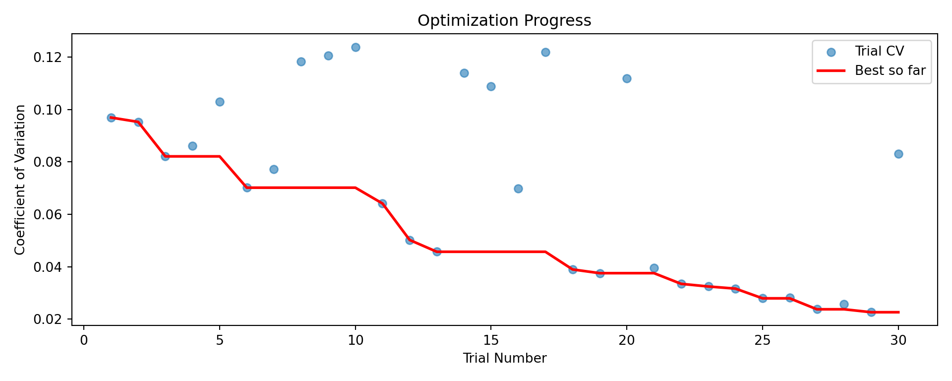

Figure 1: Optuna learns to find stable parameters over trials

Parameter Space Exploration

import pandas as pd

trial_data = []
for i, (job, _) in enumerate(result.job_results):
    cv = metrics[i] if metrics[i] < float('inf') else None
    trial_data.append({
        'grassDamage': job.parameters['grassDamage'],
        'shrubDamage': job.parameters['shrubDamage'],
        'cv': cv,
    })

df_trials = pd.DataFrame(trial_data).dropna()

plt.figure(figsize=(8, 6))

<Figure size 800x600 with 0 Axes>

scatter = plt.scatter(df_trials['grassDamage'], df_trials['shrubDamage'], 
                      c=df_trials['cv'], cmap='plasma_r', s=100, alpha=0.8)
plt.colorbar(scatter, label='CV (lower = stable)')

<matplotlib.colorbar.Colorbar object at 0x7fd95c1b3380>

plt.xlabel('Grass Damage (%)')

Text(0.5, 0, 'Grass Damage (%)')

plt.ylabel('Shrub Damage (%)')

Text(0, 0.5, 'Shrub Damage (%)')

plt.title('Parameter Space Exploration')

Text(0.5, 1.0, 'Parameter Space Exploration')

plt.tight_layout()
plt.show()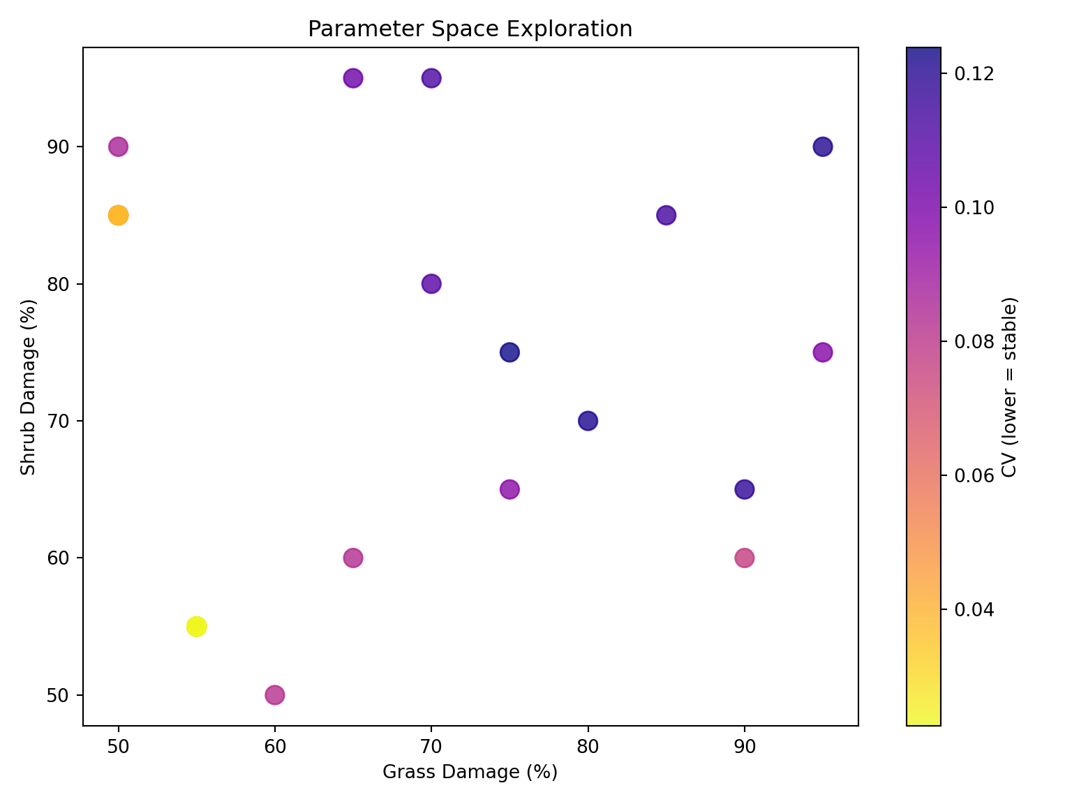

Figure 2: Parameter combinations explored, colored by stability

Step 5: Analyze Vegetation Dynamics

The real value is understanding why certain parameters are stable. We use the same analysis tools from Analysis & Visualization.

Best vs Worst Parameters

from joshpy.diagnostics import SimulationDiagnostics
from joshpy.cell_data import DiagnosticQueries

queries = DiagnosticQueries(manager.registry)
best_job = result.get_best_job()

# Note: This worst-job finding is for illustration purposes.
# In practice, you'd typically focus on the best parameters
# and use Optuna's built-in visualization tools.
finite = [(i, m) for i, m in enumerate(metrics) if m < float('inf')]
worst_idx = max(finite, key=lambda x: x[1])[0]
worst_job, _ = result.job_results[worst_idx]

fig, axes = plt.subplots(1, 2, figsize=(12, 4), sharey=True)

# Get CVs for labels
best_cv = result.best_value
worst_cv = metrics[worst_idx]

for ax, job, label, cv in [(axes[0], best_job, "BEST (stable)", best_cv), 
                            (axes[1], worst_job, "WORST (unstable)", worst_cv)]:
    df = queries.get_replicate_uncertainty("totalCover", run_hash=job.run_hash)
    ax.fill_between(df['step'], df['mean'] - df['std'], df['mean'] + df['std'], alpha=0.3)
    ax.plot(df['step'], df['mean'], linewidth=2)
    ax.axvline(50, color='gray', linestyle='--', alpha=0.5, label='Burn-in')
    ax.set_xlabel('Time Step')
    ax.set_title(f"{label}\ngrass={job.parameters['grassDamage']}%, shrub={job.parameters['shrubDamage']}%, CV={cv:.4f}")
    if ax == axes[0]:
        ax.set_ylabel('Total Cover')
        ax.legend()

<matplotlib.collections.FillBetweenPolyCollection object at 0x7fd9451017f0>
[<matplotlib.lines.Line2D object at 0x7fd945101a90>]
<matplotlib.lines.Line2D object at 0x7fd9451016a0>
Text(0.5, 0, 'Time Step')
Text(0.5, 1.0, 'BEST (stable)\ngrass=55%, shrub=55%, CV=0.0226')
Text(0, 0.5, 'Total Cover')
<matplotlib.legend.Legend object at 0x7fd945101940>
<matplotlib.collections.FillBetweenPolyCollection object at 0x7fd944f6d310>
[<matplotlib.lines.Line2D object at 0x7fd945101fd0>]
<matplotlib.lines.Line2D object at 0x7fd945101d30>
Text(0.5, 0, 'Time Step')
Text(0.5, 1.0, 'WORST (unstable)\ngrass=75%, shrub=75%, CV=0.1238')

plt.tight_layout()
plt.show()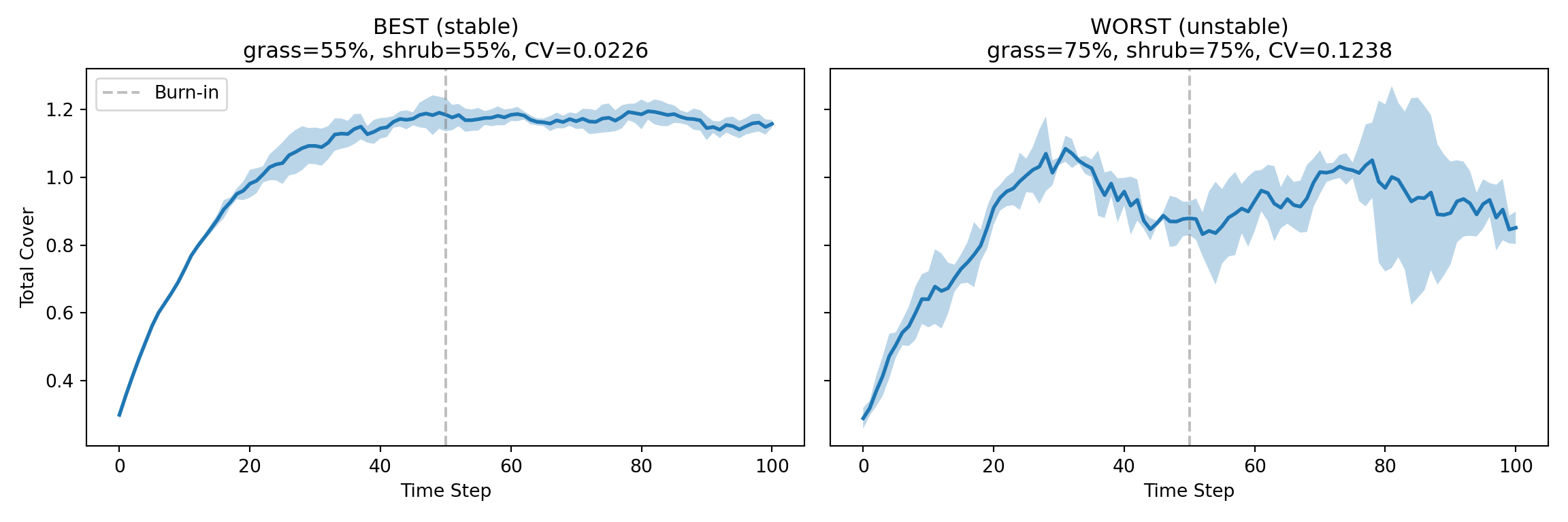

Figure 3: Stable (best) vs unstable (worst) vegetation dynamics

Species-Level Dynamics (Best Parameters)

df_grass = queries.get_replicate_uncertainty("grassCover", run_hash=best_job.run_hash)
df_shrub = queries.get_replicate_uncertainty("shrubCover", run_hash=best_job.run_hash)

fig, ax = plt.subplots(figsize=(10, 4))
ax.fill_between(df_grass['step'], df_grass['mean'] - df_grass['std'], 
                df_grass['mean'] + df_grass['std'], alpha=0.2, color='green')

<matplotlib.collections.FillBetweenPolyCollection object at 0x7fd944e1d950>

ax.plot(df_grass['step'], df_grass['mean'], color='green', linewidth=2, label='Grass')

[<matplotlib.lines.Line2D object at 0x7fd944de1a90>]

ax.fill_between(df_shrub['step'], df_shrub['mean'] - df_shrub['std'],
                df_shrub['mean'] + df_shrub['std'], alpha=0.2, color='brown')

<matplotlib.collections.FillBetweenPolyCollection object at 0x7fd944e1da90>

ax.plot(df_shrub['step'], df_shrub['mean'], color='brown', linewidth=2, label='Shrub')

[<matplotlib.lines.Line2D object at 0x7fd944de1be0>]

ax.axvline(50, color='gray', linestyle='--', alpha=0.5, label='Burn-in')

<matplotlib.lines.Line2D object at 0x7fd944de17f0>

ax.set_xlabel('Time Step')

Text(0.5, 0, 'Time Step')

ax.set_ylabel('Cover')

Text(0, 0.5, 'Cover')

ax.set_title(f"Species Dynamics (grass={best_job.parameters['grassDamage']}%, shrub={best_job.parameters['shrubDamage']}%)")

Text(0.5, 1.0, 'Species Dynamics (grass=55%, shrub=55%)')

ax.legend()

<matplotlib.legend.Legend object at 0x7fd944de1d30>

plt.tight_layout()
plt.show()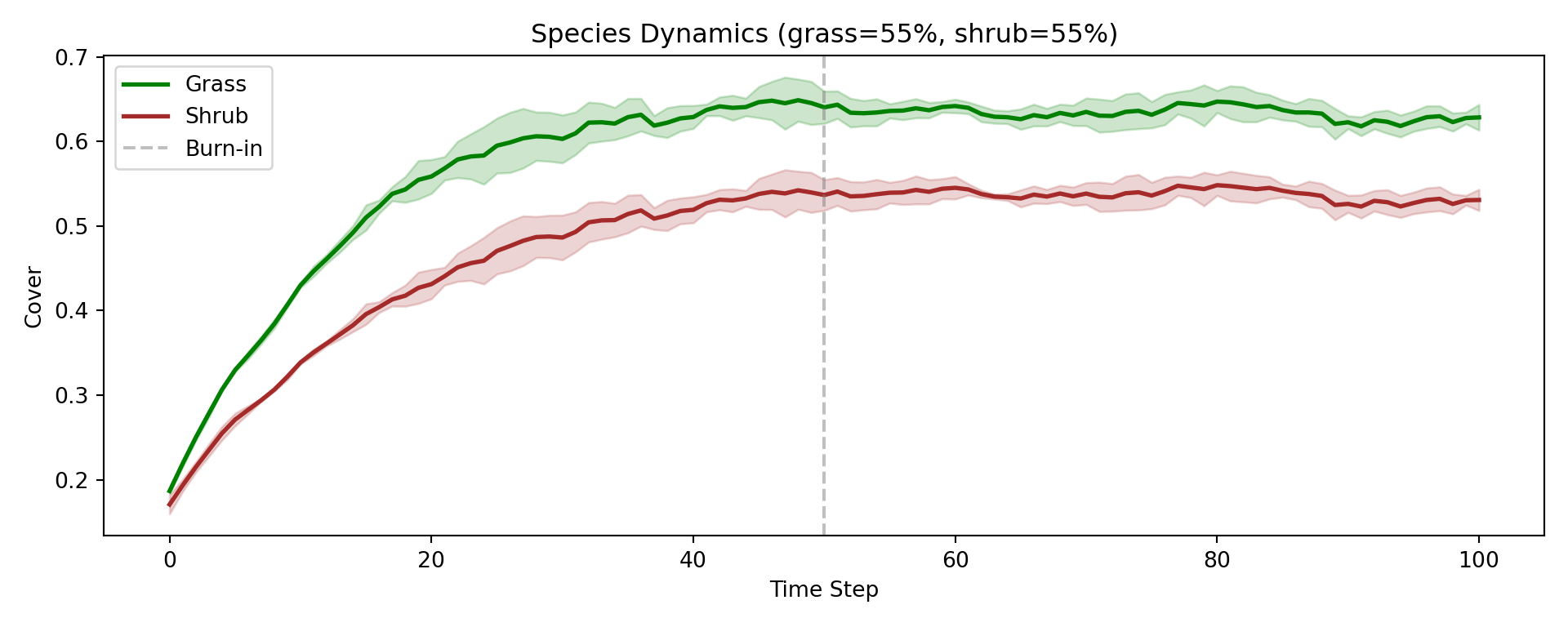

Figure 4: Grass and shrub dynamics with optimized parameters

Registry Independence

The registry produced by adaptive sweeps is identical to one from cartesian sweeps or manual workflows. All analysis tools work the same:

# Same queries work regardless of how data was generated
print(f"Variables: {manager.registry.list_export_variables()}")

Variables: ['grassCover', 'onFire', 'shrubCover', 'totalCover']

print(f"Cell data rows: {manager.registry.get_data_summary().cell_data_rows}")

Cell data rows: 227250

See Analysis & Visualization for the full analysis toolkit.

When to Use Adaptive Sweeps

Use `OptunaStrategy` when:	Use `CartesianStrategy` when:
Large parameter space	Small parameter space
Clear optimization objective	Need ALL combinations
Expensive simulations	Building response surfaces
“Good enough” parameters	Sensitivity analysis

Learn More

Optuna Documentation - Full optimization framework
TPE Sampler - Default sampler details
Analysis & Visualization - Query and visualize any registry

Cleanup

import os

manager.cleanup()
manager.close()

for f in ["adaptive_demo.duckdb", "adaptive_demo.duckdb.wal"]:
    if os.path.exists(f):
        os.remove(f)