Data Selection and Processing - Spectral Trend Database

Sample Selection¶

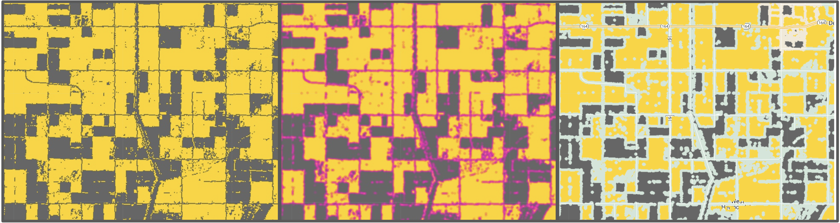
figure: neighborhood reduction of CDL corn/soy — Figure 1:Masking border values in CDL. Left: corn/soy and other, center: 60-meter radius neighborhood reduction, right: masked borders

USDA’s Crop Land Data Layer was used to create a set of corn/soy sample points, i.e. points CDL labels as (in most cases alternating between) corn or soy for at least 15 years from 2000 to 2020. In order to ensure we had “pure” pixels away from confounding effects of borders and infrastructure 60-meter radius neighborhood reductions and only kept pixel values that remained unchanged (see Figure 1). From the resulting image we selected an initial 20,000 corn/soy points.

We then used these sample points to extract yield values based on QDANN (2008-2022).

Data Processing¶

Having selected data sample points and extracted yield data, we then built a pipeline (see these scripts) to process the data and create a database (Google Big Query Dataset) containing daily-smoothed-values for 36 spectral indices, along with additional indices and annual aggregation statistics.

The resulting database is described in the docs.

The most interesting steps in the data processing are: gap-filling and smoothing, and the computation of moving average convergence divergence (divergence) indices.

Gap Filling and Smoothing¶

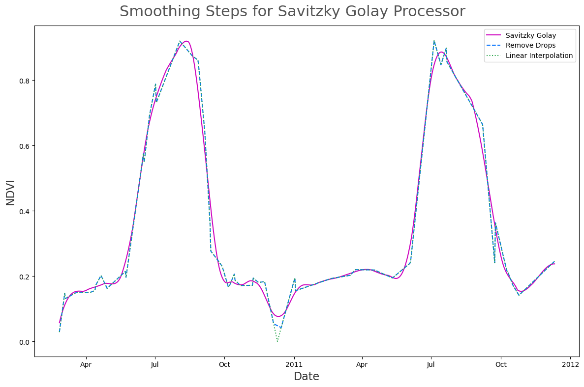
The gap filling and smoothing is managed by our savitzky_golay_processor. As illustrated in Figure 2, the following steps are taken:

Perform linear interpolation to create a daily time-series
Replace points where the time-series has a large drop using linear interpolation. Specifically, we create a smoothed curve by performing symmetrical mean smoothing over a 32 day window. We then remove, and then replace, points where the time-series data divided by the smoothed data is less than 0.5.
Apply scipy’s Savitzky Golay filter with window length 60, and polyorder 3.

Moving Average Convergence Divergence (Divergence)¶

Exponential Moving Averages (EMA), and Moving Average Convergence Divergence curves have been shown to be useful metrics in determining green-up dates. We’ve included them in our database for this specific purpose, however we also expect that the derived features may well be useful for other applications in studying agricultural trends.

\begin{aligned} macd &= ewm_a - ewm_b \\ macd_{div} &= macd - ewm_c \end{aligned}

(1)

EMA is most often written in the recursive form, $s_{t} =\alpha x_{t}+(1-\alpha )s_{t-1}$ , which is wonderful and quick when updating a series. However we are interested in examining existing series and would like to vectorize. We’ll start by expanding out the “ $t$ -th” term (using wikipedia as a reference), and then recollect our terms in a more useful form for computation:

\begin{aligned} s_{t}&=\alpha x_{t}+(1-\alpha )s_{t-1} \\[3pt] &=\alpha x_{t}+\alpha (1-\alpha )x_{t-1}+(1-\alpha )^{2}s_{t-2} \\[3pt] &=\alpha \left[x_{t}+(1-\alpha )x_{t-1}+(1-\alpha )^{2}x_{t-2}+(1-\alpha )^{3}x_{t-3}+\cdots +(1-\alpha )^{t-1}x_{1}\right]+(1-\alpha )^{t}x_{0} \ \ \ \ \text{(en.wikipedia.org/wiki/Exponential\_smoothing)}\\[3pt] &=\alpha \left[\sum_{p=0}^{t-1} x_{t-p} (1-\alpha )^{p}\right] + (1-\alpha )^{t}x_{0} \\[3pt] &=\alpha (1-\alpha )^{t} \left[\sum_{p=0}^{t-1} x_{t-p} (1-\alpha )^{p-t}\right] + (1-\alpha )^{t}x_{0} \\[3pt] &=\alpha (1-\alpha )^{t} \left[\sum_{q=1}^{t} x_{q} (1-\alpha )^{-q}\right] + (1-\alpha )^{t}x_{0}\ \ ; \ \ \ \ q\equiv(t-p) \\[3pt] &=\alpha (1-\alpha )^{t} \left[\sum_{q=1}^{t} x_{q} (1-\alpha )^{-q} + \frac{x_{0}}{\alpha}\right] \\[3pt] &=\alpha (1-\alpha )^{t} \left[\sum_{q=1}^{t} x_{q} (1-\alpha )^{-q} + \tilde{x}_{0}\right]\ \ ; \ \ \ \ \tilde{x}_{0}\equiv\frac{x_{0}}{\alpha}\\[3pt] &=\alpha (1-\alpha )^{t} \left[\sum_{q=0}^{t} \tilde{x}_{q} (1-\alpha )^{-q}\right]\ \ ; \ \ \ \ \tilde{x} \equiv [\tilde{x}_{0}, x_{1}, x_{2}, \cdots ]\\[3pt] \end{aligned}

(2)

We can now write this in vector form where $s = \left[ s_0, s_1, \cdots s_{N} \right]$ :

\begin{aligned} s&=\alpha\ (1-\alpha)^{\overline{N}} \text{CUMSUM}[\tilde{x} \times (1-\alpha)^{-\overline{N}} ] \\[3pt] \overline{N}&\equiv[0,1,2,\cdots N]\ \ ; \ \ \ \ N+1 = \text{size of }\tilde{x} \end{aligned}

(3)

This final form can be easily implemented in python, as we have done here.

It’s worth noting however that $(1-\alpha)^{\pm t}$ terms quickly become infinitesimal or expload leading to problematic overflow errors. Depending on your choice of α they appear around $t \sim 2000$ . Our series are much smaller than this and its therefore not an issue. Nonetheless, it’s worth noting how we might fix the issue. Naively we could just replace these terms with 0 at sufficiently large $t$ . If we want to only keep terms of order $t_{max}$ we need to make sure that we only keep the terms in the summation who’s total power is less than $t_{max}$ . The most straightforward way to this is to return to the “geometric” form we’ve copied from wikipedia. Then for a given α and max-precision compute $t_{max}$ and force all terms with $t>t_{max}$ to zero. A better approach might be to consider the “effective window size” (span in the below code). The idea is that the vast majority of the contributions come from this window. If we took some batch size of M * span for sufficiently large M (let’s say 50) we could calculate EWM in sequential batches, avoid overflow errors with negligible contributions. The (relative) scale of these approximation would be $(1-\alpha)^{M*span}$

References¶

Gao, F., Anderson, M., Daughtry, C., Karnieli, A., Hively, D., & Kustas, W. (2020). A within-season approach for detecting early growth stages in corn and soybean using high temporal and spatial resolution imagery. Remote Sensing of Environment, 242, 111752. 10.1016/j.rse.2020.111752

Spectral Trend Database

Examples

Notebooks

Examples