Examples - Spectral Trend Database

Before diving into how the data was produced and processed, let’s take a look at a few examples of how to use the spectral_trend_database module.

Querying the Database¶

The data is in a big-query database, and so can be accessed using the big-query api.

Source:

Examples

client = bq.Client()
sql = f'SELECT sample_id, date, ndvi FROM `{BQ_PREFIX}.RAW_INDICES_V1` LIMIT 3'
resp = client.query(sql)
resp.to_dataframe()

Here is the same query using query.QueryConstructor

Source:

Examples

qc = query.QueryConstructor('RAW_INDICES_V1', table_prefix=BQ_PREFIX)
qc.select('sample_id', 'date', 'ndvi')
qc.limit(3)
df = query.run(sql=qc.sql())

print(qc.sql(),'\n')
df

The real benefit, however, is in constructing SQL queries with multiple JOIN and WHERE statements. Here is a more complicated request collecting spectral index data from 2010-2013 for a subset of sample_ids:

Source:

Examples

qc = query.QueryConstructor(
        'SAMPLE_POINTS', 
        table_prefix=BQ_PREFIX,
        using=['sample_id'],  
        how='inner')
qc.join('MACD_INDICES_V1')
qc.join('SMOOTHED_INDICES_V1', 'sample_id', 'date')
qc.where_in(sample_id=sample_ids)
qc.where('SMOOTHED_INDICES_V1', year=2010, year_op='>=')
qc.where('SMOOTHED_INDICES_V1', year=2014, year_op='<')
qc.orderby('date', table='MACD_INDICES_V1')
df = query.run(sql=qc.sql(), print_sql=True)
example_id = df.sample_id.sample().iloc[0]
rows = df[df.sample_id == example_id]
rows

Parsing the data¶

Using the utils module we can easily turn these rows into xarray-datasets to parse and interact with the data.

Source:

Examples

ATTR_COLS = COLUMN_NAMES[SAMPLES_TABLE]
ds = utils.rows_to_xr(rows, attr_cols=ATTR_COLS)
fig, ax = plt.subplots(figsize=(12, 2))
ds.savi.plot(ax=ax)
display(ds)

And then filter by dates

Source:

Examples

START_MMDD = '04-01'
END_MMDD = '10-15'

def growing_season_for_year(ds, year):
    return ds.sel(dict(date=slice(f'{year}-{START_MMDD}', f'{year}-{END_MMDD}')))

_ds = growing_season_for_year(ds, 2012)
fig, ax = plt.subplots(figsize=(4, 2))
_ds.savi.plot(ax=ax)
display(_ds)

Computations and Visualizations¶

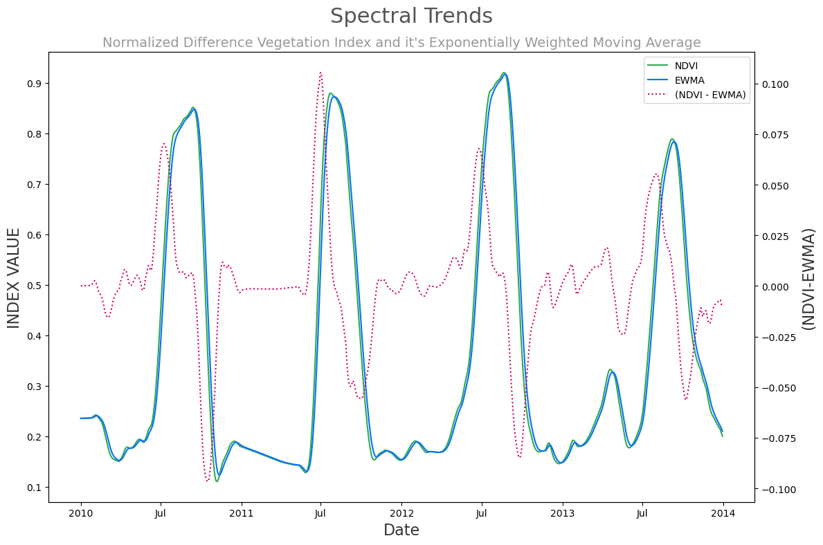
This workflow allows us to efficiently perform computations and visualize the data. Here’s a quick visualization of NDVI and it’s exponentially weighted moving average (EWMA). Additionally we have added to the visualization a computed trend, namely the difference between the NDVI and it’s EWMA, in order to elucidate the magnitude of the shift.

Source:

Examples

fig, ax = plt.subplots(figsize=(12, 8))
ax2 = ax.twinx()

(ds.ndvi - ds.ndvi_ema_b).plot(color='#cc0066', linestyle='dotted', label='(NDVI - EWMA)', ax=ax2)
ds.ndvi.plot(color='#32a852', label='NDVI', ax=ax)
ds.ndvi_ema_b.plot(color='#0473fd', label='EWMA', ax=ax)

plt.title(TITLE,fontsize=TITLE_FONT_SIZE,color=TITLE_CLR)
plt.suptitle(SUPTITLE,fontsize=SUPTITLE_FONT_SIZE,color=SUPTITLE_CLR)

ax.set_ylabel('INDEX VALUE', fontsize=LABEL_FONT_SIZE, color=LABEL_CLR)
ax2.set_ylabel('(NDVI-EWMA)', fontsize=LABEL_FONT_SIZE, color=LABEL_CLR)
ax.set_xlabel('Date', fontsize=LABEL_FONT_SIZE, color=LABEL_CLR)
twinx_legend(ax, ax2)

plt.tight_layout()

Spectral Trend Database

Data Selection and Processing