Examples - Spectral Trend Database

date: 2025-01-15
authors:
    - name: Brookie Guzder-Williams
affiliations:
    - University of California Berkeley, The Eric and Wendy Schmidt Center for Data Science & Environment
license: CC-BY-4.0

This notebook gives examples of how to use DSE’s Spectral Trend Database. In particular we look at:

Querying the Database
Parsing the data
Visualizing the data

IMPORTS¶

from pprint import pprint
import matplotlib.pyplot as plt
from google.cloud import bigquery as bq
from spectral_trend_database.config import config as c
from spectral_trend_database import query
from spectral_trend_database import utils

CONFIG¶

BQ_PREFIX = 'dse-regenag.SpectralTrendDatabase'
SAMPLE_FRAC = 0.0005
YEAR_START = 2008
YEAR_END = 2020
START_MMDD = '11-01'
END_MMDD = START_MMDD
ATTR_COLS = [
    'sample_id',
    'lon',
    'lat']
LIST_ATTRS = [
    'year',
    'biomass',
    'crop_type']
CHART_DATA_PATH = 'spectral_trends.chart_data.json'

HELPER METHODS¶

def print_list(lst, max_len=7, view_size=3, sep=', ', connector=' ... '):
    size = len(lst)
    if size <= max_len:
        lst_str = sep.join(lst)
    else:
        head = sep.join(lst[:view_size])        
        tail = sep.join(lst[-view_size:])
        lst_str = f'{head}{connector}{tail}  [{size}]'
    print(lst_str)

def line(marker='-', length=100):
    print(marker*length)

DATABSE QUERIES¶

STDB DATABASE INFO¶

First we’ll take a quick peak at the what is in the STDB database

SAMPLES_TABLE = 'SAMPLE_POINTS'
YIELD_TABLE = 'QDANN_YIELD'
SMOOTHED_INDICES_TABLE = 'SMOOTHED_INDICES_V1'
IDENT_DATE_COLUMNS = ['sample_id', 'year', 'date']

COLUMN_NAMES = {}
print('DATABASE INFO')
line()
table_names = query.table_names()
print('TABLES:')
pprint(table_names)
for table_name in [SAMPLES_TABLE, YIELD_TABLE, SMOOTHED_INDICES_TABLE]:
    COLUMN_NAMES[table_name] = query.column_names(table_name, run_query=True)
    print(f'\n{table_name}:')
    print_list(COLUMN_NAMES[table_name])
line()

DATABASE INFO
----------------------------------------------------------------------------------------------------
TABLES:
['QDANN_YIELD',
 'SMOOTHED_INDICES_V1',
 'INDICES_STATS_V1',
 'RAW_INDICES_V1',
 'SAMPLE_POINTS',
 'INDICES_STATS_V1_GROWING_SEASON',
 'INDICES_STATS_V1_OFF_SEASON',
 'CDL_CROP_TYPE',
 'MACD_INDICES_V1']

SAMPLE_POINTS:
AWATER, ALAND, LSAD ... h3_4, NAME, h3_9  [20]

QDANN_YIELD:
qdann_crop_label, qdann_crop_type, nb_years, biomass, year, sample_id

SMOOTHED_INDICES_V1:
si1, rvi, si ... savi, rdvi, year  [45]
----------------------------------------------------------------------------------------------------

INDICES = [c for c in COLUMN_NAMES[SMOOTHED_INDICES_TABLE] if c not in IDENT_DATE_COLUMNS]
print_list(INDICES)

si1, rvi, si ... blue, savi, rdvi  [42]

USING BIG QUERY¶

The data is in a big-query database, and so can be accessed using the big-query api

client = bq.Client()
sql = f'SELECT sample_id, date, ndvi FROM `{BQ_PREFIX}.RAW_INDICES_V1` LIMIT 3'
resp = client.query(sql)
resp.to_dataframe()

QueryConstructor and Helper Methods¶

Using big-query directly is easy enough. However, constructing SQL statements with lots of JOIN and WHERE statements can be painful. To handle this we’ve developed a simple QueryConstructor. Additionaly we’ve added a few convience methods so the user never needs to use the big-query python module directly. You’ve already seen two of them: query.table_names and query.column_names.

Let’s start by reproducing the SQL in our simple example above

qc = query.QueryConstructor('RAW_INDICES_V1', table_prefix=BQ_PREFIX)
qc.select('sample_id', 'date', 'ndvi')
qc.limit(3)
df = query.run(sql=qc.sql())

print(qc.sql(),'\n')
df

Now we’ll create an more complicated request using the sample_ids from the above example.

First I’ll need to select the sample_ids of interest

qc = query.QueryConstructor('SAMPLE_POINTS', table_prefix=BQ_PREFIX)
qc.select('DISTINCT sample_id')
qc.limit(3)
qc.sql()

'SELECT DISTINCT sample_id FROM `dse-regenag.SpectralTrendDatabase.SAMPLE_POINTS` LIMIT 3'

locales_df = query.run(sql=qc.sql())
sample_ids = locales_df.sample_id.tolist()
sample_ids

['9yrxd2cmudy', '9yry7n3rvb5', '9yryeyjyhre']

qc = query.QueryConstructor(
        'SAMPLE_POINTS', 
        table_prefix=BQ_PREFIX,
        using=['sample_id'],  
        how='inner')
qc.join('MACD_INDICES_V1')
qc.join('SMOOTHED_INDICES_V1', 'sample_id', 'date')
qc.where_in(sample_id=sample_ids)
qc.where('SMOOTHED_INDICES_V1', year=2010, year_op='>=')
qc.where('SMOOTHED_INDICES_V1', year=2014, year_op='<')
qc.orderby('date', table='MACD_INDICES_V1')
df = query.run(sql=qc.sql(), print_sql=True)
example_id = df.sample_id.sample().iloc[0]
rows = df[df.sample_id == example_id]
rows

PARSING THE DATA¶

We can easily turn these rows into xarray-datasets to more easily parse interact with the data.

ATTR_COLS = COLUMN_NAMES[SAMPLES_TABLE]
ds = utils.rows_to_xr(rows, attr_cols=ATTR_COLS)
fig, ax = plt.subplots(figsize=(12, 2))
ds.savi.plot(ax=ax)
display(ds)

xarrays can easily be filtered by dates

START_MMDD = '04-01'
END_MMDD = '10-15'

def growing_season_for_year(ds, year):
    return ds.sel(dict(date=slice(f'{year}-{START_MMDD}', f'{year}-{END_MMDD}')))

_ds = growing_season_for_year(ds, 2012)
fig, ax = plt.subplots(figsize=(4, 2))
_ds.savi.plot(ax=ax)
display(_ds)

Computations and Visulaizations¶

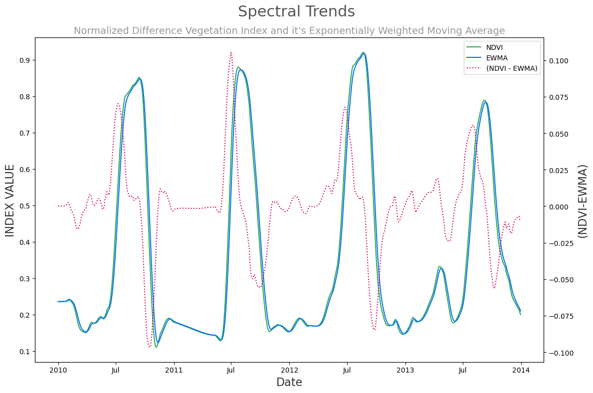
SUPTITLE = 'Spectral Trends'
TITLE = 'Normalized Difference Vegetation Index and it\'s Exponentially Weighted Moving Average'
SUPTITLE_FONT_SIZE = 22
SUPTITLE_CLR = '#555'
TITLE_FONT_SIZE = 14
TITLE_CLR = '#999'
LABEL_FONT_SIZE = 16
LABEL_CLR = '#333'

def twinx_legend(ax, ax2):
    lines, labels = ax.get_legend_handles_labels()
    lines2, labels2 = ax2.get_legend_handles_labels()
    return ax2.legend(lines + lines2, labels + labels2, loc=1)

fig, ax = plt.subplots(figsize=(12, 8))
ax2 = ax.twinx()

(ds.ndvi - ds.ndvi_ema_b).plot(color='#cc0066', linestyle='dotted', label='(NDVI - EWMA)', ax=ax2)
ds.ndvi.plot(color='#32a852', label='NDVI', ax=ax)
ds.ndvi_ema_b.plot(color='#0473fd', label='EWMA', ax=ax)

plt.title(TITLE,fontsize=TITLE_FONT_SIZE,color=TITLE_CLR)
plt.suptitle(SUPTITLE,fontsize=SUPTITLE_FONT_SIZE,color=SUPTITLE_CLR)

ax.set_ylabel('INDEX VALUE', fontsize=LABEL_FONT_SIZE, color=LABEL_CLR)
ax2.set_ylabel('(NDVI-EWMA)', fontsize=LABEL_FONT_SIZE, color=LABEL_CLR)
ax.set_xlabel('Date', fontsize=LABEL_FONT_SIZE, color=LABEL_CLR)
twinx_legend(ax, ax2)

plt.tight_layout()

Spectral Trend Database

Data Selection and Processing

Notebooks

Gap Filling & Smoothing