Vector
points, lines, polygons
FILETYPES
There are lots of file-types!
- csv (point data)
- shapefile
- geojson
- geopackage
- flatgeobuf
- geoparquet
Read more about them here: guide
line()
print('parq, json, gpkg, (shp)')
line()
print('SAVE')
%time gdf.to_parquet('fires.parquet')
%time gdf.to_file('fires.json', driver="GPKG")
%time gdf.to_file("fires.gpkg", layer='calfires', driver="GPKG")
line()
print('READ')
%time gdf_parq = gpd.read_parquet('fires.parquet')
%time gdf_json = gpd.read_file('fires.json', driver="GPKG")
%time gdf_gpkg = gpd.read_file("fires.gpkg", layer='calfires', driver="GPKG")
line()
print('SIZE')
print('parq:', Path('fires.parquet').stat().st_size)
print('json:', Path('fires.json').stat().st_size)
print('gpkg:', Path('fires.gpkg').stat().st_size)
print('shp: ', directory_size(FIRES))
---------------------------------------------------------------------------
parq, json, gpkg, (shp)
---------------------------------------------------------------------------
SAVE
CPU times: user 219 ms, sys: 54 ms, total: 273 ms
Wall time: 285 ms
CPU times: user 345 ms, sys: 349 ms, total: 693 ms
Wall time: 818 ms
CPU times: user 351 ms, sys: 350 ms, total: 700 ms
Wall time: 835 ms
---------------------------------------------------------------------------
READ
CPU times: user 175 ms, sys: 73.6 ms, total: 249 ms
Wall time: 242 ms
CPU times: user 202 ms, sys: 46.5 ms, total: 248 ms
Wall time: 249 ms
CPU times: user 202 ms, sys: 42 ms, total: 244 ms
Wall time: 245 ms
---------------------------------------------------------------------------
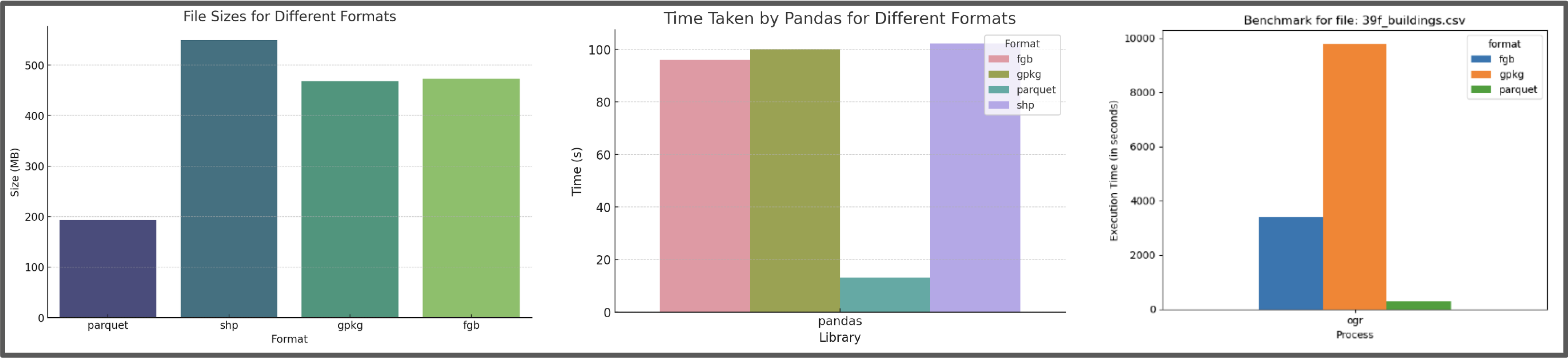
SIZE
parq: 95010603
json: 108892160
gpkg: 108892160
shp: 117379885
However, this isn’t capturing the performace gains captured by the columnar data + row grouping. A detailed performance comparison can be found here: https://
GEOPANDAS
We’ll start by loading historical CalFires data from 1898 through 2021. An updated version of this data can be found here.
gdf = gpd.read_file(FIRES)
gdf = gdf.to_crs(epsg=4326)
print('data shape:', gdf.shape)
print('example:')
row = gdf[(gdf.GIS_ACRES > 100) & (gdf.YEAR_=='2021')].sample().iloc[0]
display(row.geometry)
rp.pprint(row.to_dict())ax = gdf.plot()
txt = ax.set_title('CalFires Data')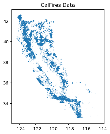
LEAFMAP
"Leafmap is a Python package for interactive mapping and geospatial analysis with minimal coding in a Jupyter environment.
Leafmap supports multiple mapping backends, including ipyleaflet, folium, kepler-gl, pydeck, and bokeh. You can switch between these backends to create maps with different visualization styles and capabilities."
Our modest fires dataset has 16327 polygons is too big for leafmap. One could probably simplify the polygons, but we’ll take the approach of filtering the data for 2016-2021 resulting in 2553 polygons (about 16% of the entire dataset). After about 20 seconds you will see a map.
_gdf = gdf[gdf.year>2015]
leafmap_map = leafmap.Map(zoom=ZOOM)
leafmap_map.center = MAP_CENTER
leafmap_map.add_gdf(_gdf, layer_name='Fires', fill_colors=["red", "yellow", "green", "orange"])
leafmap_map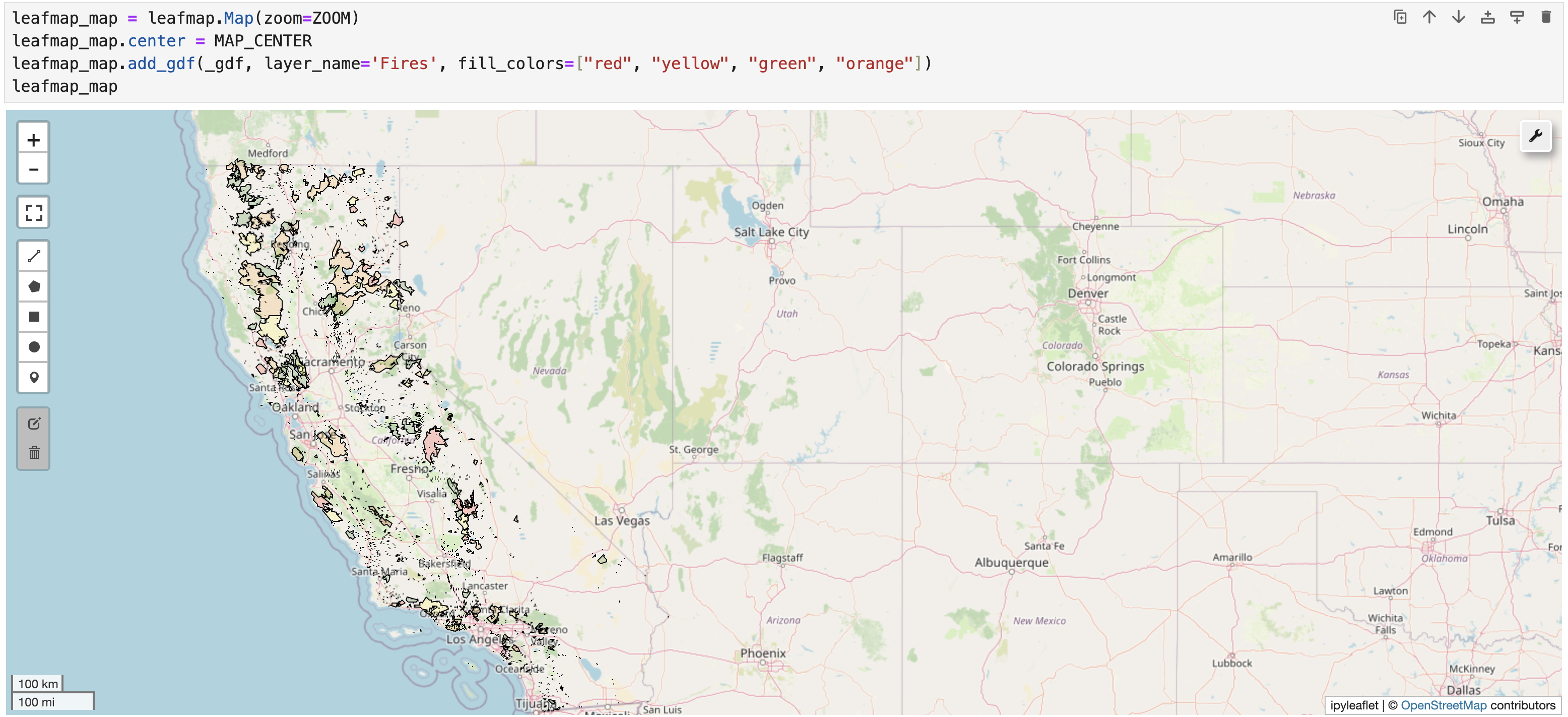
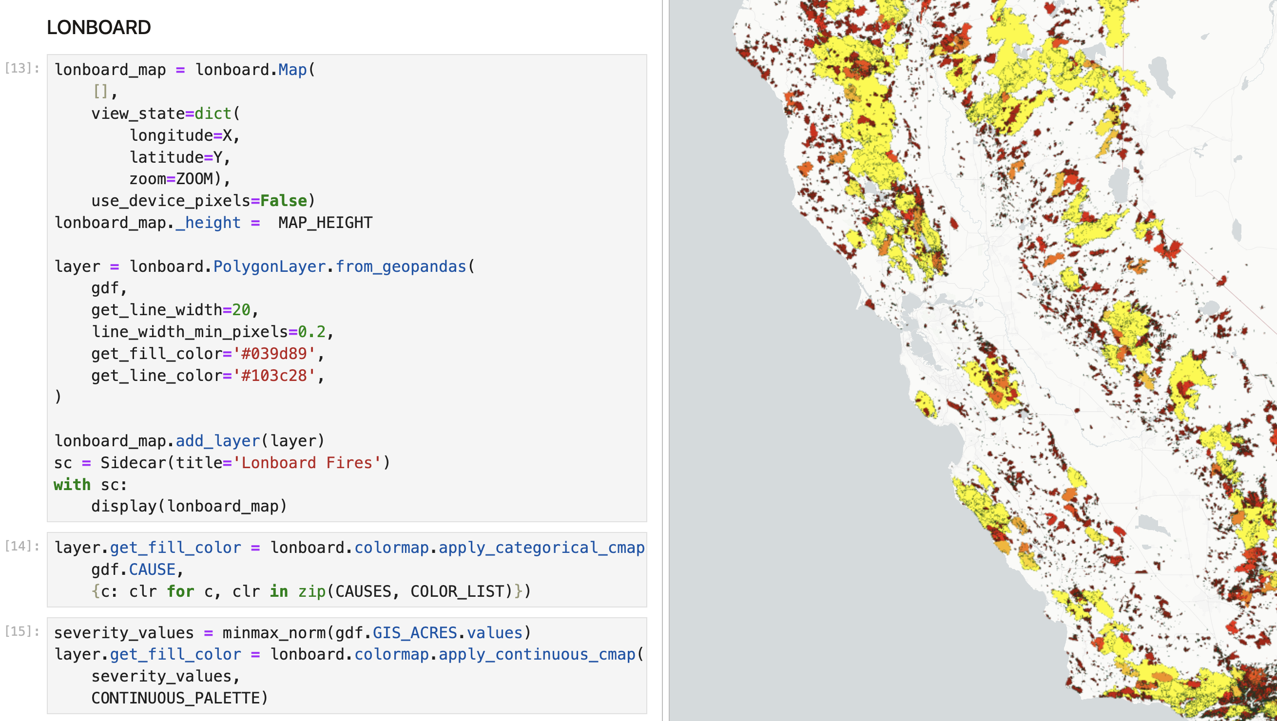
LONBOARD
"A Python library for fast, interactive geospatial vector data visualization in Jupyter.
Building on cutting-edge technologies like GeoArrow and GeoParquet in conjunction with GPU-based map rendering, Lonboard aims to enable visualizing large geospatial datasets interactively through a simple interface."
Here is a great discussion on Matt Forrest’s GIS youtube show.
A quick overview:
- GEOARROW: enables sharing data between libaries (python to javascript). As an example GDAL speed up file reading 26x by using geoarrow on the backend
- GEOPARQUET: ipyleaflet & pydeck first byte object write to geojson. geoparquet will keep it in bytes. In ipyleaflet and pydeck a 300 million point database gets converted to 700MB geojson. geoparquet will be 60MB for the same data.
- DECK-GL: python rendering with the GPU
Here we’ll plot the full dataset [1898-2021] using longboard. After about 4 seconds you’ll see a map