Raster Data
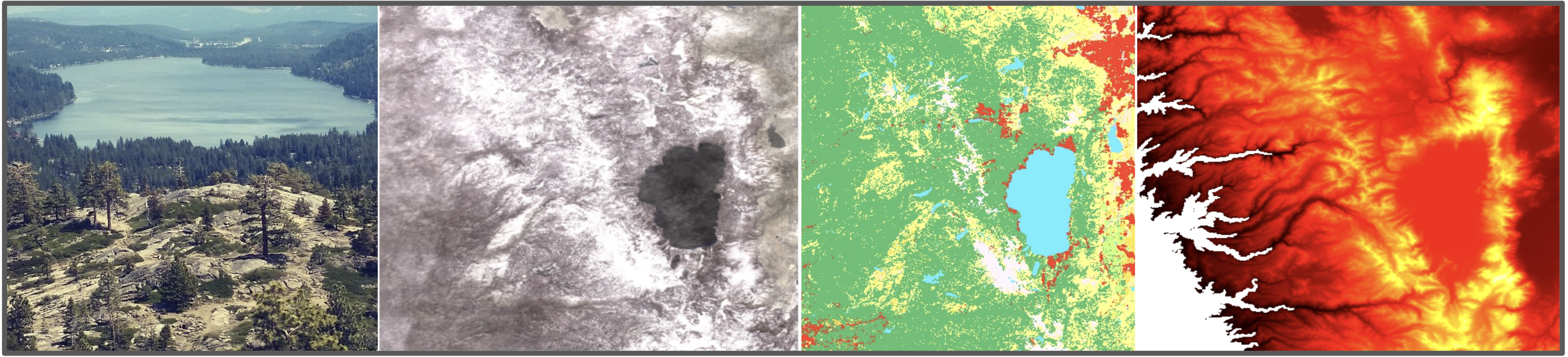
Raster data is simply pixels with values. This can be an ordinary photograph, but much more. For example a digital elevation model may have 3-bands (elevation, slope, aspect), landuse classification will give a single int band representing the type of land use, and perhaps additional band representing other details such as classification confidence
GEOTIFF
What makes a GeoTiff different than a traditional image.
- more bands: sentinel-2 for instance has 12 optical bands + others) as opposed to RGB.
- adds geospatial data
- projection and coordinate-reference-system (CRS)
- location (affine transform)
READING DATA WITH RASTERIO
def read_rio(path: str) -> tuple[np.ndarray, dict[str, Any]]:
    """ read a geotiff using rasterio """
    with rio.open(path,'r') as src:
        profile = src.profile
        arr = src.read()
    return arr, profile

dem_arr, dem_profile = read_rio(PATHS[0])
s2_arr, s2_profile = read_rio(PATHS[1])
line()
print('Sentinel-2:', s2_arr.shape)
rp.pprint(s2_profile)
line()
visualize_arrays(s2_arr, dem_arr)COMMON COORDINATE REFERENCE SYSTEMS
- EPSG:4326: A global CRS (on WGS84) using latitude and longitude coordinates in degrees
- UTM (EPSG:32HZZ): UTM CRS divide the northern and southern hemisphere up into 60 zones of 6 longitude. The EPSG codes are broken up 32 (UTM) [6,7] (north or south) [01-60] zone. Each EPSG uses x and y coordinates measured in meters.
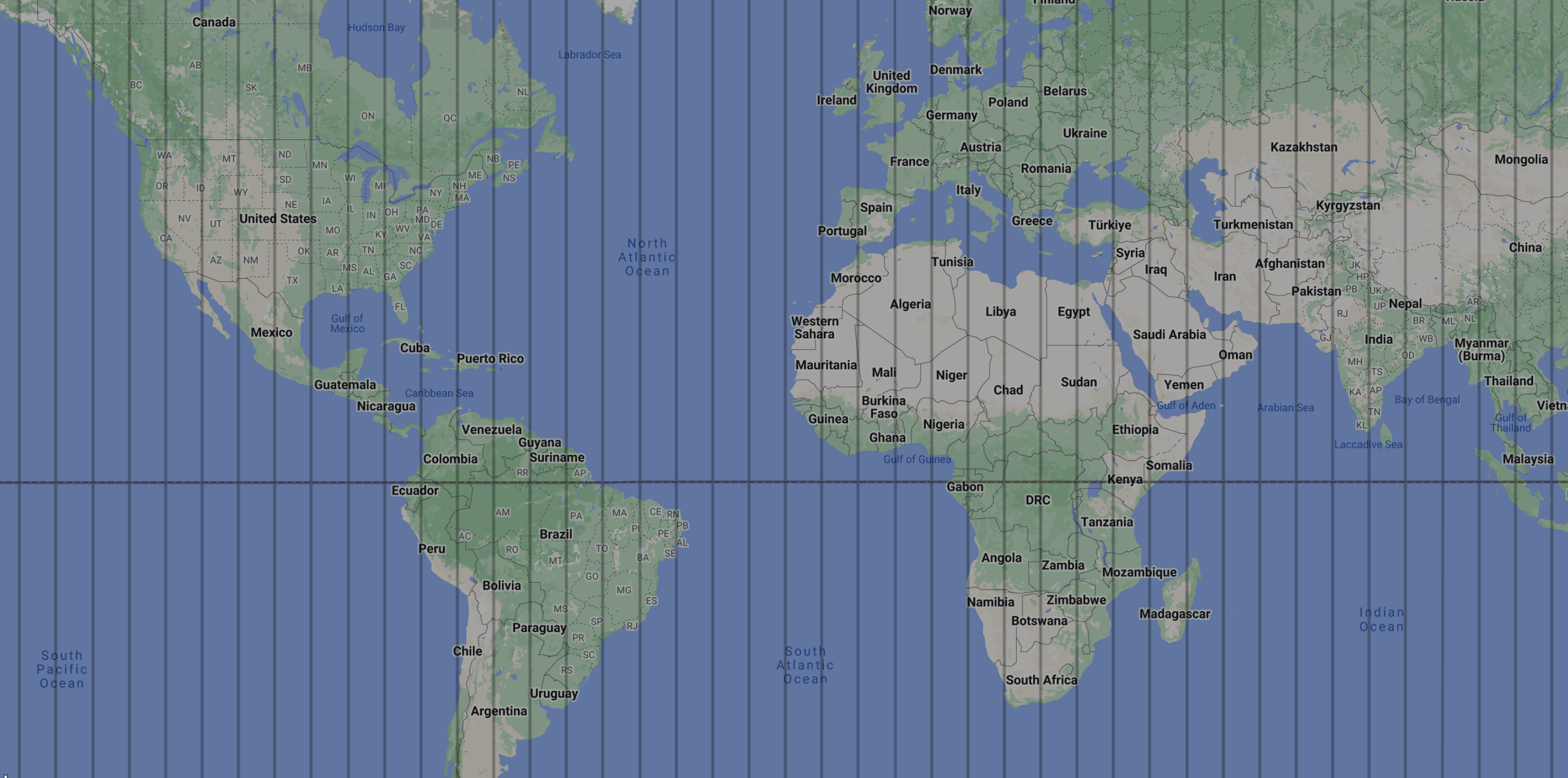
- EPSG:3857: A global CRS (on WGS84) using x and y coordinates in meters. This is a great choice for visualizations (online maps) but is only accurate near the equator and therefore shouldn’t be used for calculations
STRUCTURE OF AFFINE TRANSFORMATIONS
READING DATA WITH RIOXARRAY
rio-xarray allows you to read the data directly into an xr.DataArray.
Some advantages:
- we now have access to the lat, lon values
da.x,y - we also have access to the band-names
da.long_namewhose order corresponds with the returned numpy array
da = rxr.open_rasterio(PATHS[1])
print('array equality:', np.array_equal(da.data, s2_arr, equal_nan=True))
daBy transforming the xr.DataArray to a xr.Dataset the adavantages become more manifest
def bandify_data_array(da: xr.DataArray, bands: Union[list[str], str]='long_name') -> xr.Dataset:
    """ transform data-array to dataset with band-valued data_vars """
    if isinstance(bands, str):
        bands = list(da.attrs[bands])
    return xr.Dataset(
        data_vars={b: (['y', 'x'], da.data[i]) for i, b in enumerate(bands)},
        coords=dict(
            x=("x", da.x.data),
            y=("y", da.y.data)
        ),
        attrs=da.attrs)

ds = bandify_data_array(da)
(ds.B8-ds.B4).plot()
plt.title('NDVI')
plt.show()
dsMAPTILES
For interactive mapping often broken into map tiles: a url endpoint http://.../{z}/{x}/{y}, where z is the “ZOOM” level, and x and y are integers defining a tile on a coordinate grid.
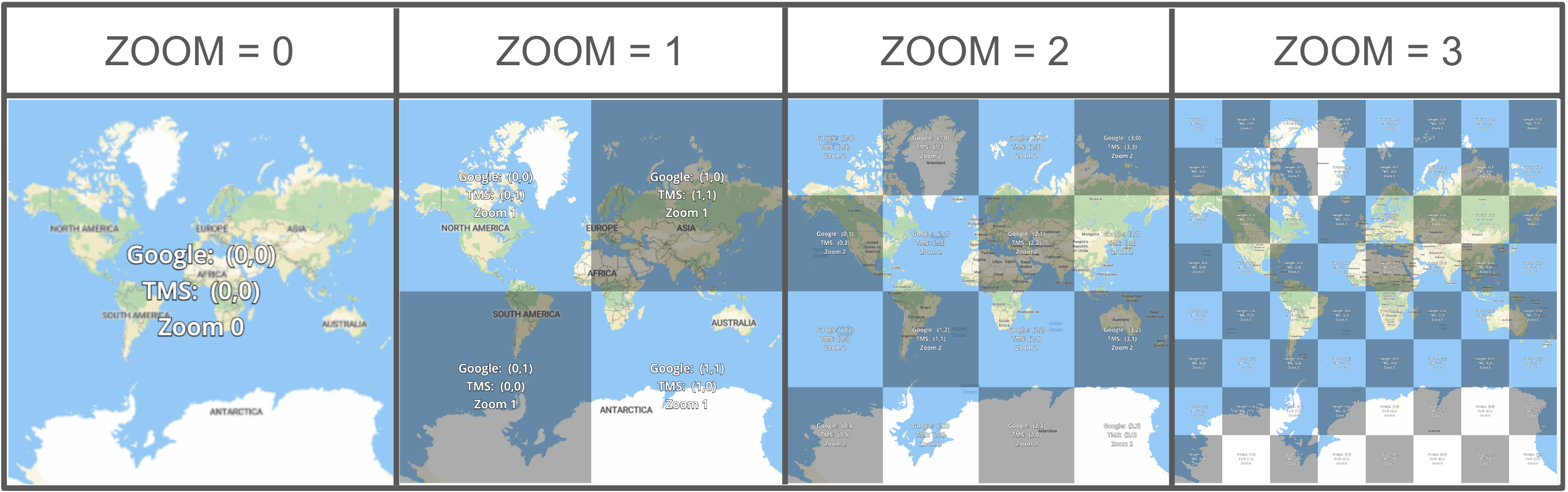
(a)zoom levels 0-3 (src https://docs.maptiler.com/google-maps-coordinates-tile-bounds-projection)
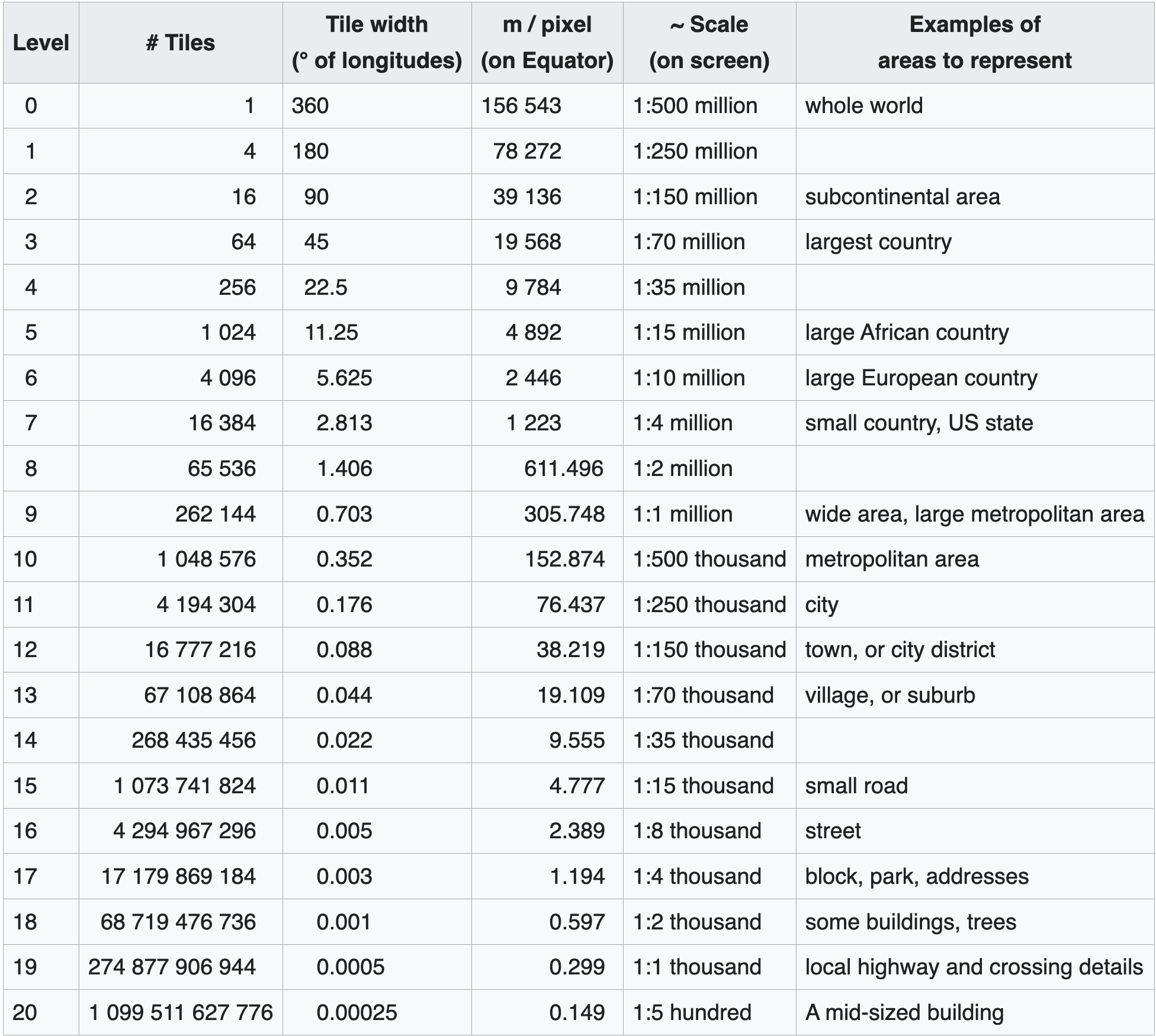
(b)number of tiles and tile sizes per zoom level (src: https://wiki.openstreetmap.org/wiki/Zoom_levels)
rio-tiler is a Rasterio plugin to read mercator tiles from Cloud Optimized GeoTIFF’s. Used to create serverless tiles server with lambda-tiler. As an example maptiles/app.py creates a dynamic-tiler from cloud optimized geotiffs
Whats a Cloud Optimized GeoTiff (COG)?
“A Cloud Optimized GeoTIFF (COG) is a regular GeoTIFF file, aimed at being hosted on a HTTP file server, with an internal organization that enables more efficient workflows on the cloud”
A (over) simplified way to think about this is a a geotiff that allows get requests so that
- one can get parts of the pixels without fetching all the data
- the aggregation at different zoom levels is already computed
COGs can be created from tifs using rio-cogeo
!rio cogeo create ../data/raster/tahoe-mean-s2-20210101_20210301.tif ../data/raster/cogs/tahoe-mean-s2-20210101_20210301.tifReading input: /Users/brookieguzder-williams/code/dse/map_something/repo/data/raster/tahoe-mean-s2-20210101_20210301.tif
[####################################] 100%
Adding overviews...
Updating dataset tags...
Writing output to: ../data/raster/cogs/tahoe-mean-s2-20210101_20210301.tif
ZARR
Similar to COGs but uses a multiple file approach (metadata files + one file per data chunk) whereas uses a single file approach
They can be created from
.zattrs
.zgroup
.zmetadata
├── AOT
│   ├── 0.0
│   ├── 0.1
│   ├── 0.2
...
│   └── 9.7
├── B1 ...
├── B11 ...
├── B12 ...
├── B2 ...
├── B3 ...
├── B4 ...
├── B5 ...
├── B6 ...
├── B7 ...
├── B8 ...
├── B8A ...
├── B9 ...
├── MSK_CLASSI_CIRRUS ...
├── MSK_CLASSI_OPAQUE ...
├── MSK_CLASSI_SNOW_ICE ...
├── MSK_CLDPRB ...
├── MSK_SNWPRB ...
├── QA10 ...
├── QA20 ...
├── QA60 ...
├── SCL ...
├── TCI_B ...
├── TCI_G ...
├── TCI_R ...
├── WVP ...
├── x
│   └── 0
└── y
    └── 0
MAP SOMETHING!
Let’s make a map (finally). It’s easy using leafmap
- leafmap has three plotting backends: folium, ipyleaflet, and here-map-widget-for-jupyter.
- provides an interactive graphical user interface (GUI) for loading geospatial datasets without any coding.
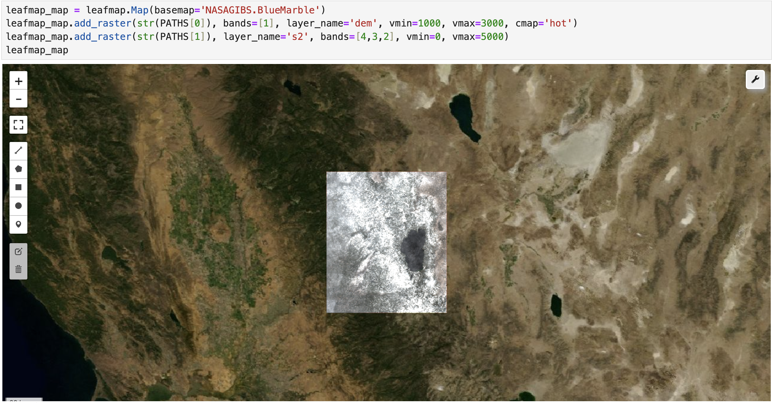
leafmap serving raster layers directly from cogs
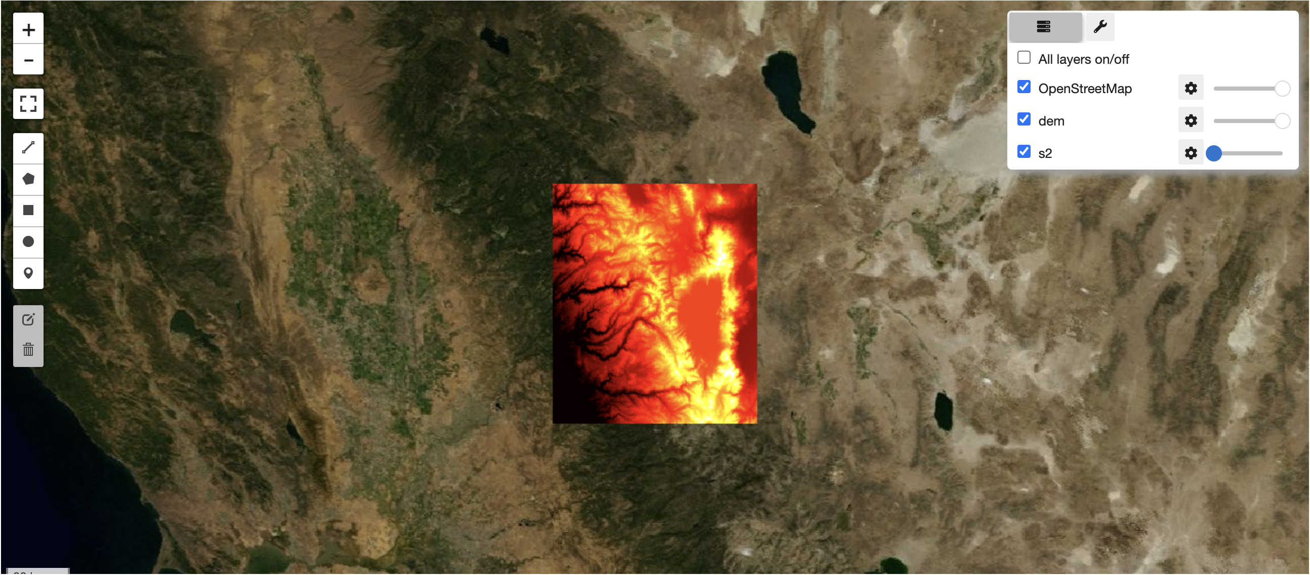
hiding sentinel-2 layer to reveal dem