Eureka Fire Exploration

Published

June 11, 2025

Setup

Load required libraries

library(tidyverse)        
library(sf)            
library(raster)          
library(exactextractr)    
library(leaflet)         
library(htmlwidgets)     
library(viridis)        
library(readr)
library(scales)
library(ggridges)
library(RColorBrewer)

Read data

veg_data <- st_read(dsn = "../../shared_inputs/jotrgeodata.gpkg",layer = "JOTR_VegPolys", 
                    quiet = TRUE)

# Read fire severity (raster)
rbr_rast <- raster("inputs/refined_rbr.tif")

Interactive map of fire location

# Build two palette functions (to force descending order in leaflet legend) :
pal      <- colorNumeric("plasma", domain = values(rbr_rast), 
                         na.color = "transparent")
pal_rev  <- colorNumeric("plasma", domain = values(rbr_rast), 
                         na.color = "transparent", reverse = TRUE)

# Draw the map
leaflet(options = leafletOptions(attributionControl = TRUE)) %>%
  addProviderTiles("CartoDB.Positron") %>% # Use the reversed palette for the raster itself
  addRasterImage(rbr_rast, colors = pal_rev, opacity = 0.6,project = FALSE) %>% # Use the normal palette + label transform for the legend
  addLegend(position= "bottomright", pal = pal, values = values(rbr_rast), 
            title = "RBR value",
            labFormat = labelFormat(transform = function(x) sort(x, decreasing = TRUE)))

Static RBR map with grid

# Turn the RasterLayer into a data.frame
rbr_df <- as.data.frame(rasterToPoints(rbr_rast))
colnames(rbr_df) <- c("x", "y", "RBR")

ggplot(rbr_df, aes(x = x, y = y, fill = RBR)) +
  geom_raster() +
  scale_fill_viridis_c(option = "plasma", direction = -1,  na.value  = "transparent",
    name = "RBR value", limits  = c(-0.2, 0.5), breaks = seq(-0.2, 0.5, by = 0.1)) +
  coord_equal() +
  labs(title = "Refined Relative Burn Ratio (RBR)", x = NULL, y = NULL) +
  theme_minimal(base_size = 12) +
  theme(panel.grid.major = element_blank(),
        panel.grid.minor = element_blank(),
        panel.border = element_rect(fill = NA, color = "black", size = 0.5),
        axis.ticks = element_line(color = "black"),
        axis.text = element_text(color = "black"),
        panel.background = element_blank(),
        legend.position = "right")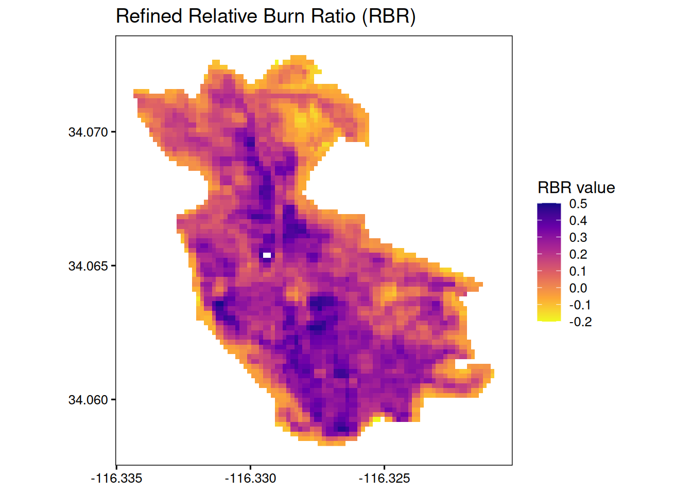

Reproject raster to match vegetation data and calculate area

For the purpose of this analysis, we reprojected the fire severity raster into NAD83 / UTM zone 11N to match the vegetation map, which may introduce some imprecision of sentinel 2 cells

# Grab the vector’s CRS as a PROJ4/WKT string
vec_crs <- st_crs(veg_data)$proj4string

# Reproject the raster to that CRS
#    - use method="bilinear" for continuous data
rbr_to_vec_crs <- projectRaster(rbr_rast, crs = vec_crs, method = "bilinear")

Extract fire perimeter from raster

# Polygonize all positive, non‐NA cells from the reprojected raster, convert to sf und merge into a single boundary polygon
fire_boundary <- rasterToPolygons(rbr_to_vec_crs, fun = function(x) !is.na(x) & x > 0, 
                          dissolve = TRUE) %>%
  st_as_sf() %>%
  st_union() 

# Write to file
if (file.exists("outputs/fire_perimeter/severity_to_fire_perimeter.shp")) {
  file.remove("outputs/fire_perimeter/severity_to_fire_perimeter.shp")
}

[1] TRUE

st_write(fire_boundary, "outputs/fire_perimeter/severity_to_fire_perimeter.shp")

Writing layer `severity_to_fire_perimeter' to data source 
  `outputs/fire_perimeter/severity_to_fire_perimeter.shp' using driver `ESRI Shapefile'
Writing 1 features with 0 fields and geometry type Multi Polygon.

#convert reprojected raster to dataframe
rbr_to_vec_crs_df <- as.data.frame(rasterToPoints(rbr_to_vec_crs))
colnames(rbr_to_vec_crs_df) <- c("x", "y", "RBR")

#plot fire severity with generated fire boundary 
ggplot() +
  geom_raster(data = rbr_to_vec_crs_df, aes(x = x, y = y, fill = RBR)) +
  geom_sf(data = fire_boundary, fill = NA, color = "black", linewidth = 0.8) +
  scale_fill_viridis_c(option = "plasma", direction = -1,  na.value  = "transparent",
    name = "RBR value", limits  = c(-0.2, 0.5), breaks = seq(-0.2, 0.5, by = 0.1)) +
  coord_sf() +
  labs(title = "Burned Area Boundary (RBR > 0)", x = NULL, y = NULL) +
  theme_minimal(base_size = 12) +
  theme(panel.grid.major = element_blank(),
        panel.grid.minor = element_blank(),
        panel.border = element_rect(fill = NA, color = "black", size = 0.5),
        axis.ticks = element_line(color = "black"),
        axis.text = element_text(color = "black"),
        axis.text.x = element_text(angle = 45, hjust = 1),
        panel.background = element_blank(),
        legend.position = "right")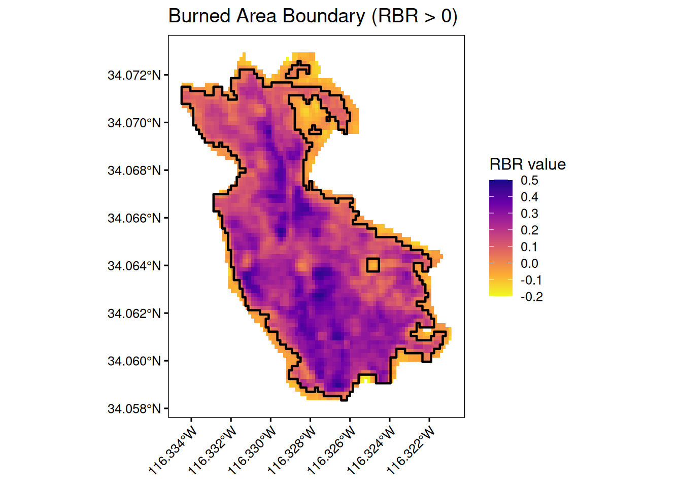

Clip vegetation data to fire boundary and ummarize vegetation types within fire boundary

# Calculate area per vegetation type polygon
clipped_veg <- st_intersection(veg_data, fire_boundary) %>%
  mutate(area_ha = as.numeric(st_area(.) / 10000))  # m² → ha

# Summarize hectares by vegetation type
veg_summary <- clipped_veg %>%
  st_set_geometry(NULL) %>%          # drop geometry for speed
  group_by(MapUnit_Name) %>%
  summarise(veg_ha = sum(area_ha, na.rm = TRUE), .groups = "drop") %>%
  mutate(pct_of_total = 100 * veg_ha / sum(veg_ha)) %>%# total area can be calculated in pipe
  bind_rows(tibble(MapUnit_Name = "Total Burned Area", 
                   veg_ha = sum(clipped_veg$area_ha), pct_of_total = 100)) %>%
  arrange(desc(pct_of_total))

# write out
write_csv(veg_summary, "outputs/veg_burned_summary.csv")

# show table
knitr::kable(veg_summary)

MapUnit_Name	veg_ha	pct_of_total
Total Burned Area	87.1560000	100.0000000
Singleleaf Pinyon / Muller Oak Woodland Association	48.4475490	55.5871644
Joshua Tree - California Juniper / Nevada Ephedra Woodland Association	19.3109766	22.1567954
Muller Oak - California Buckwheat - Narrowleaf Goldenbush Shrubland Association	9.5698538	10.9801434
California Juniper / Blackbush Woodland Association	5.1160438	5.8699846
Red Brome - Mediterranean Grass Semi-Natural Herbaceous Stands	3.0957694	3.5519865
Mojave Yucca - Blackbush Shrubland Association	1.3421753	1.5399689
Joshua Tree / Blackbush Woodland Association	0.2736322	0.3139568

Assertions

# After creating fire_boundary
fire_boundary_area <- st_area(fire_boundary) %>% units::set_units("ha")
cat("Total fire boundary area (ha):", fire_boundary_area, "\n")

Total fire boundary area (ha): 87.156

# After clipping vegetation
total_veg_area <- sum(clipped_veg$area_ha)
cat("Sum of vegetation areas within fire (ha):", total_veg_area, "\n")

Sum of vegetation areas within fire (ha): 87.156

# Assert that these are approximately equal (within small tolerance for computational differences)
stopifnot(abs(as.numeric(fire_boundary_area) - total_veg_area) < 0.1)

Map vegetation types and their area within fire boundary

# Join summary back to clipped polygons
clipped_joined <- clipped_veg %>%
    dplyr::left_join(dplyr::select(veg_summary, MapUnit_Name, veg_ha, pct_of_total),
    by = "MapUnit_Name")

# Create an ordered factor of vegetation types
ordered_types <- veg_summary %>%
  filter(MapUnit_Name != "Total Burned Area") %>%
  arrange(desc(pct_of_total)) %>%
  pull(MapUnit_Name)

# Pick colors from the Set3 palette
n_types   <- length(ordered_types)
set3_cols <- brewer.pal(n = max(3, n_types), "Set3")[1:n_types]
names(set3_cols) <- ordered_types

# Build legend labels without the word “Association”
legend_labels <- veg_summary %>%
  filter(MapUnit_Name != "Total Burned Area") %>%
  mutate(clean_name = MapUnit_Name %>% # remove “Association” and clean up whitespace
           str_remove_all("Association") %>%
           str_squish(),
         label = sprintf("%s\n%.1f ha (%.1f%%)",
                         clean_name,
                         veg_ha,
                         pct_of_total)) %>%
  pull(label) %>%
  set_names(ordered_types)  # keep the same factor levels for mapping

# Total burned area for caption
total_fire_ha <- veg_summary %>%
  filter(MapUnit_Name == "Total Burned Area") %>%
  pull(veg_ha)

# wrap your legend labels to ~30 chars per line
legend_labels_wrapped <- legend_labels %>% 
  lapply(str_wrap, width = 30) %>% 
  unlist(use.names = TRUE)

#plot
ggplot(clipped_joined) +
  geom_sf(aes(fill = factor(MapUnit_Name, levels = ordered_types)),
          color = "gray80", size = 0.2) +
  scale_fill_manual(values = set3_cols, labels = legend_labels_wrapped, 
                    name   = "Vegetation Type:\nArea (ha) & % of Total") +
  coord_sf(crs = st_crs(4326)) +   # keep geographic graticule if you like
  labs(title   = "", caption = sprintf("Total Burned Area: %.1f ha", total_fire_ha)) +
  theme_minimal(base_size = 10) +
  theme(panel.grid.major = element_blank(),
        panel.grid.minor = element_blank(),
        panel.border = element_rect(fill = NA, color = "black", size = 0.5),
        panel.background = element_blank(),
        axis.text.x = element_text(angle = 45, hjust = 1),  # ← slanted labels
        axis.text.y = element_text(size = 8),
        axis.ticks = element_line(color = "black"),
        axis.title = element_blank(),
        legend.position = "right",
        legend.text = element_text(size = 9),
        legend.title = element_text(size = 10, face = "bold"),
        legend.key.height = unit(1, "cm"),     # ↑ match the guide keyheight
        legend.spacing.y = unit(1, "cm"), 
        plot.caption = element_text(hjust  = 2.5, margin = margin(b = 2)))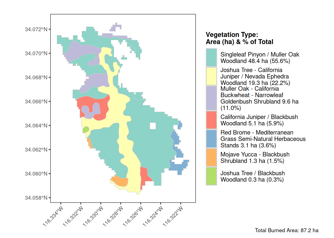

Summary statistics of fire severity by vegetation type

merged_units_veg <- clipped_veg %>%
  dplyr::select(MapUnit_Name, SHAPE) %>% 
  group_by(MapUnit_Name) %>%
  summarise(do_union = TRUE, .groups = "drop")

 # Compute per-polygon stats
clipped_stats <- merged_units_veg %>%
  mutate(min_RBR = exact_extract(rbr_to_vec_crs, ., "min",progress = FALSE),
         max_RBR = exact_extract(rbr_to_vec_crs, ., "max",progress = FALSE),
         mean_RBR = exact_extract(rbr_to_vec_crs, ., "mean",progress = FALSE),
         median_RBR = exact_extract(rbr_to_vec_crs, ., "median",progress = FALSE),
         sd_RBR = exact_extract(rbr_to_vec_crs, ., "stdev",progress = FALSE),
         n_pixels = exact_extract(rbr_to_vec_crs, ., "count",progress = FALSE))


#  Reorder to your preferred sequence
ordered_veg <- c("Singleleaf Pinyon / Muller Oak Woodland Association",
                 "Joshua Tree - California Juniper / Nevada Ephedra Woodland Association",
                 "Muller Oak - California Buckwheat - Narrowleaf Goldenbush Shrubland Association",
                 "California Juniper / Blackbush Woodland Association",
                 "Red Brome - Mediterranean Grass Semi-Natural Herbaceous Stands",
                 "Mojave Yucca - Blackbush Shrubland Association",
                 "Joshua Tree / Blackbush Woodland Association")

severity_summary <- clipped_stats %>%
  slice(match(ordered_veg, MapUnit_Name))  %>%
  st_set_geometry(NULL)


#Write
write_csv(severity_summary, "outputs/severity_veg_summary.csv")

# View results
knitr::kable(
  severity_summary)

MapUnit_Name	min_RBR	max_RBR	mean_RBR	median_RBR	sd_RBR	n_pixels
Singleleaf Pinyon / Muller Oak Woodland Association	0.0006178	0.4402448	0.1876000	0.1880521	0.0980251	1794.35364
Joshua Tree - California Juniper / Nevada Ephedra Woodland Association	0.0006927	0.4703166	0.2723719	0.2855063	0.0918550	715.22137
Muller Oak - California Buckwheat - Narrowleaf Goldenbush Shrubland Association	0.0010206	0.4248829	0.1628162	0.1470451	0.0935087	354.43903
California Juniper / Blackbush Woodland Association	0.0026619	0.4724639	0.2085815	0.2073311	0.0872869	189.48311
Red Brome - Mediterranean Grass Semi-Natural Herbaceous Stands	0.0012685	0.2954386	0.1017317	0.0921144	0.0693485	114.65813
Mojave Yucca - Blackbush Shrubland Association	0.0026019	0.4074306	0.1493467	0.1252532	0.1119501	49.71020
Joshua Tree / Blackbush Woodland Association	0.0150545	0.4356584	0.2343643	0.2361572	0.0997474	10.13452

Plot fire severity by vegetation type

# Extract pixel values per polygon directly
vals_list <- extract(rbr_to_vec_crs, merged_units_veg)

# Build long tibble
vals_df <- tibble(MapUnit_Name = merged_units_veg$MapUnit_Name, value = vals_list) %>%
  unnest(cols = c(value)) %>%
  filter(!is.na(value)) %>%
  mutate(MapUnit_Name = factor(MapUnit_Name, levels = ordered_veg))

# Prepare colors & wrapped labels
set3_cols      <- brewer.pal(length(ordered_veg), "Set3")
names(set3_cols) <- ordered_veg
labels_wrapped <- str_wrap(ordered_veg, width = 25)

#  Plot
ggplot(vals_df, aes(x = MapUnit_Name, y = value, fill = MapUnit_Name)) +
  geom_violin(trim = FALSE, color = "black", alpha = 0.8) +
  stat_summary(fun = median, geom = "point", size = 1.5, color = "black") +
  scale_fill_manual(values = set3_cols, guide = FALSE) +
  scale_x_discrete(labels = labels_wrapped) +
  labs(x = NULL,
       y = "Refined Relative Burn Ratio (RBR)",
       title = "Fire Severity Distribution by Vegetation Type\n(ordered left → right by % burned area)") +
  theme_minimal(base_size = 12) +
  theme(axis.text.x = element_text(angle = 45, hjust = 1, size = 10),
        panel.grid.major.y = element_line(color = "grey80", linetype = "dashed"),
        panel.grid.major.x = element_blank(),
        panel.grid.minor = element_blank(),
        plot.title = element_text(hjust = 0.5, size = 14))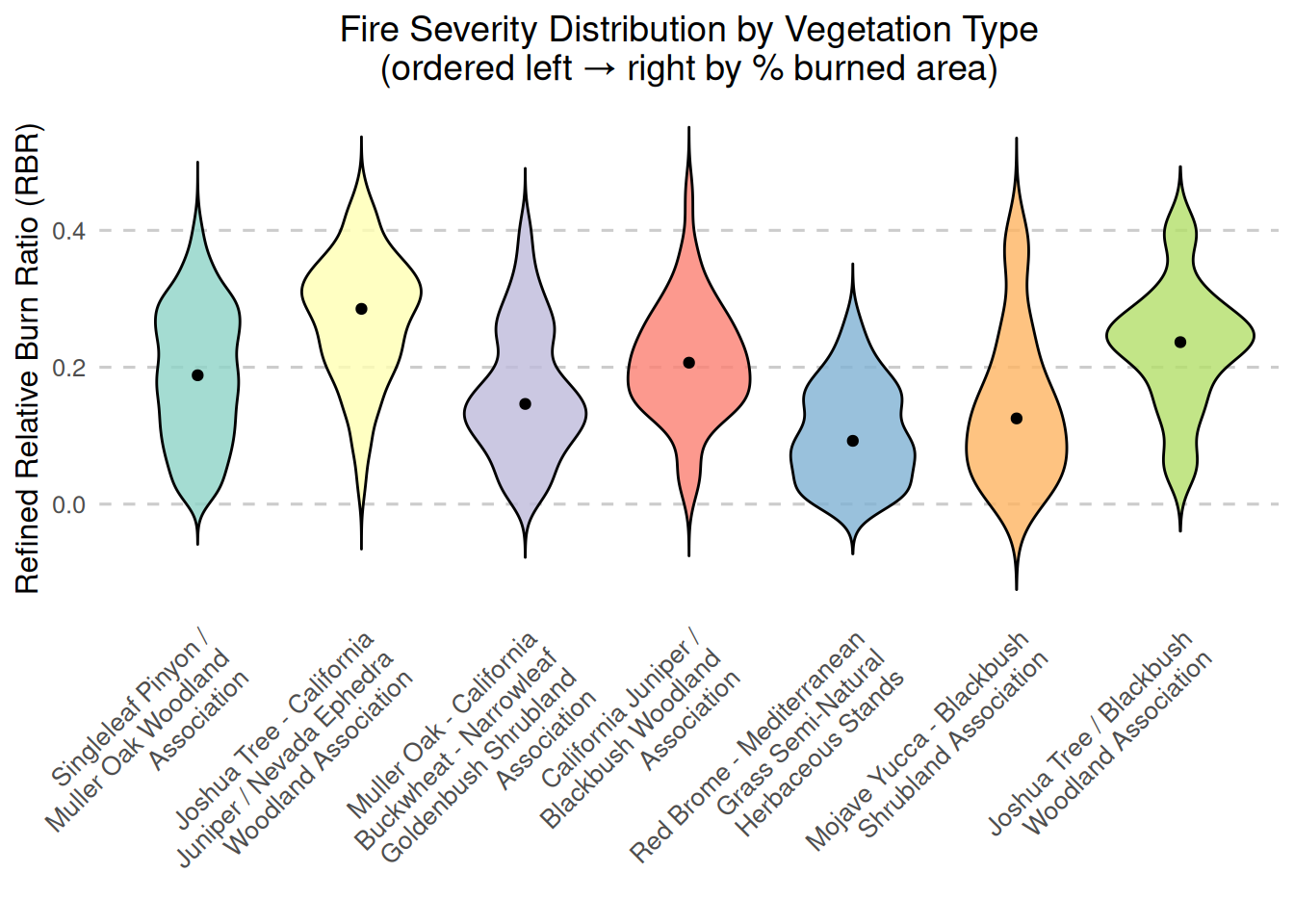

Load Historical Fires

# Read the historic‐fires shapefile
fire_hist <- st_read("../../shared_inputs/HistFires_JOTR_MOJA/FindExistingLocationsOutput.shp") %>% # Reproject into EPSG:26911 (NAD83 / UTM zone 11N)
  st_transform(26911)

Map historical fires and Eureka fire boundary

#  palette for all years —
fire_years <- sort(unique(fire_hist$YEAR_))
pal_fire <- setNames(viridis(n = length(fire_years), option = "turbo"), fire_years)

# create a 100% buffer around the Eureka fire polygon
#    (buffer distance = max(width, height) of its bbox)
fb <- fire_boundary %>%
  st_union() %>% # ensure single geometry
  {
    bb  <- st_bbox(.)
    dist <- max(bb$xmax - bb$xmin, bb$ymax - bb$ymin)
    st_buffer(., dist) 
  }

# find which historic fires intersect that buffer
visible_yr <- fire_hist %>%
  filter(st_intersects(., fb, sparse = FALSE)) %>%
  pull(YEAR_) %>%
  unique() %>%
  sort()

# plot
ggplot() +
  geom_sf(data = fire_hist, aes(fill = factor(YEAR_)), colour = "black", 
          size = 0.2, alpha = 0.6) +
  geom_sf(data = fire_boundary, fill   = NA, colour = "red", size = 1) +
  coord_sf(xlim = st_bbox(fb)[c("xmin", "xmax")], ylim = st_bbox(fb)[c("ymin", "ymax")],
           expand = FALSE) +
  scale_fill_manual(name   = "Fire Year", values = pal_fire, breaks = visible_yr) +
  labs(title = "Historical Fires & Eureka Fire Boundary") +
  theme_void(base_size = 14) +
  theme(legend.position = c(0.85, 0.85),
        legend.background = element_rect(fill = "white", color = "grey80"),
        legend.title = element_text(face = "bold", size = 10),
        legend.text = element_text(size = 8),
        plot.title = element_text(hjust = 0.5, size = 16))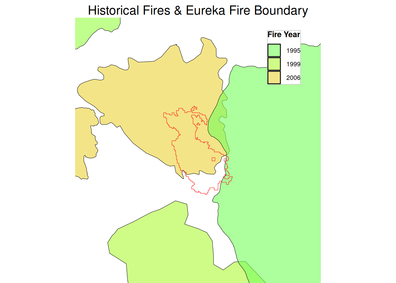

Summary statistics of fire severity by historical fire

#  Intersection of historic fires & Eureka boundary
burned_overlap <- st_intersection(fire_hist, fire_boundary)

# Burned stats by YEAR_ + FIRE_NAME (still sf)
burned_stats <- burned_overlap %>%
  mutate(min_RBR = exact_extract(rbr_to_vec_crs, ., "min",progress = FALSE),
         max_RBR = exact_extract(rbr_to_vec_crs, ., "max",progress = FALSE),
         mean_RBR = exact_extract(rbr_to_vec_crs, ., "mean",progress = FALSE),
         sd_RBR = exact_extract(rbr_to_vec_crs, ., "stdev",progress = FALSE),
         area_ha = st_area(geometry)/10000) %>%
  dplyr::select(FIRE_NAME, YEAR_, min_RBR, max_RBR, mean_RBR, sd_RBR, area_ha)


#  Unburned remainder stats (also an sf)
unburned_stats <- st_sf(FIRE_NAME = "Previously Unburned", YEAR_ = 0,
                        geometry  = st_sfc(st_difference(st_union(fire_boundary), st_union(burned_overlap))),
    crs       = st_crs(fire_boundary)) %>%
  mutate(min_RBR = exact_extract(rbr_to_vec_crs, ., "min",progress = FALSE),
         max_RBR = exact_extract(rbr_to_vec_crs, ., "max",progress = FALSE),
         mean_RBR = exact_extract(rbr_to_vec_crs, ., "mean",progress = FALSE),
         sd_RBR = exact_extract(rbr_to_vec_crs, ., "stdev",progress = FALSE),
         area_ha = st_area(geometry)/10000) %>%
  dplyr::select(FIRE_NAME, YEAR_, min_RBR, max_RBR, mean_RBR, sd_RBR, area_ha)


#  Combine
full_fire_history <- bind_rows(burned_stats, unburned_stats)

# Plot:
# plot(full_fire_history["FIRE_NAME"])

# Drop geometry and fix the NA‐row
full_fire_history_table <- full_fire_history %>%
  st_set_geometry(NULL) %>%
  mutate(YEAR_  = if_else(is.na(YEAR_), 0L, YEAR_),
         FIRE_NAME = if_else(is.na(FIRE_NAME), "Unburned", FIRE_NAME))


#Write
write_csv(full_fire_history_table, "outputs/severity_fire_history.csv")

# Display
knitr::kable(
  full_fire_history_table)

FIRE_NAME	YEAR_	min_RBR	max_RBR	mean_RBR	sd_RBR	area_ha
WHISPERING PINES	2006	0.0006178	0.4724639	0.1930639	0.1028691	63.612771 [m^2]
COVINGTON	1995	0.0012685	0.2601025	0.0969125	0.0643561	2.529986 [m^2]
Previously Unburned	0	0.0006927	0.4672158	0.2392190	0.0964592	21.013242 [m^2]

Assertions

burned_area_sum <- sum(as.numeric(st_area(burned_overlap))) / 10000
unburned_area <- as.numeric(st_area(unburned_stats)) / 10000
total_calculated_area <- burned_area_sum + unburned_area

cat("Sum of historical burned areas (ha):", burned_area_sum, "\n")

Sum of historical burned areas (ha): 66.14276

cat("Unburned area (ha):", unburned_area, "\n")

Unburned area (ha): 21.01324

cat("Total calculated area (ha):", total_calculated_area, "\n")

Total calculated area (ha): 87.156

cat("Total fire boundary area (ha):", as.numeric(fire_boundary_area), "\n")

Total fire boundary area (ha): 87.156

# Check these are approximately equal
stopifnot(abs(total_calculated_area - as.numeric(fire_boundary_area)) < 0.1)

Summary statistics fire severity by vegetation type & fire history

# overlay veg × fire
veg_hist <- st_intersection(
  merged_units_veg["MapUnit_Name"],
  burned_overlap[c("FIRE_NAME","YEAR_")]
)

# compute per‐polygon RBR stats (still sf)
veg_hist_stats <- veg_hist %>%
  mutate(min_RBR   = exact_extract(rbr_to_vec_crs, ., "min",progress = FALSE),
         max_RBR   = exact_extract(rbr_to_vec_crs, ., "max",progress = FALSE),
         mean_RBR  = exact_extract(rbr_to_vec_crs, ., "mean",progress = FALSE),
         sd_RBR    = exact_extract(rbr_to_vec_crs, ., "stdev",progress = FALSE),
         area_ha   = as.numeric(st_area(.)) / 10000)


# build the “previously unburned” pieces
burned_union  <- st_union(burned_overlap)
veg_unburned  <- st_difference(merged_units_veg, burned_union) %>%
  filter(!st_is_empty(.))

# compute stats on unburned (still sf)
veg_unburned_stats <- veg_unburned %>%
  mutate(min_RBR = exact_extract(rbr_to_vec_crs, ., "min",progress = FALSE),
         max_RBR = exact_extract(rbr_to_vec_crs, ., "max",progress = FALSE),
         mean_RBR  = exact_extract(rbr_to_vec_crs, ., "mean",progress = FALSE),
         sd_RBR = exact_extract(rbr_to_vec_crs, ., "stdev",progress = FALSE),
         area_ha = as.numeric(st_area(.)) / 10000, 
         FIRE_NAME = "Previously Unburned",YEAR_ = 0L)

#  bind burned + unburned
full_veg_history <- bind_rows(veg_hist_stats, veg_unburned_stats) %>%
  mutate(MapUnit_Name = factor(MapUnit_Name, levels = ordered_veg, ordered = TRUE),
         FIRE_NAME = factor(FIRE_NAME, levels = c("WHISPERING PINES","COVINGTON","Previously Unburned"), ordered = TRUE)) %>%
  arrange(MapUnit_Name, FIRE_NAME)%>%
  st_set_geometry(NULL)


#Write
write_csv(full_veg_history, "outputs/severity_veg_firehist.csv")

#show
knitr::kable(
  full_veg_history)

MapUnit_Name	FIRE_NAME	YEAR_	min_RBR	max_RBR	mean_RBR	sd_RBR	area_ha
Singleleaf Pinyon / Muller Oak Woodland Association	WHISPERING PINES	2006	0.0006178	0.4402448	0.1708716	0.0969081	35.6587526
Singleleaf Pinyon / Muller Oak Woodland Association	COVINGTON	1995	0.0041944	0.2381883	0.1056019	0.0555091	0.0596381
Singleleaf Pinyon / Muller Oak Woodland Association	Previously Unburned	0	0.0041544	0.4136359	0.2348462	0.0848635	12.7291584
Joshua Tree - California Juniper / Nevada Ephedra Woodland Association	WHISPERING PINES	2006	0.0137789	0.4703166	0.2665175	0.0905737	13.9284866
Joshua Tree - California Juniper / Nevada Ephedra Woodland Association	Previously Unburned	0	0.0006927	0.4672158	0.2875216	0.0934025	5.3824901
Muller Oak - California Buckwheat - Narrowleaf Goldenbush Shrubland Association	WHISPERING PINES	2006	0.0010206	0.4248829	0.1628162	0.0935087	9.5698538
California Juniper / Blackbush Woodland Association	WHISPERING PINES	2006	0.0062844	0.4724639	0.2111886	0.0886525	3.9139999
California Juniper / Blackbush Woodland Association	Previously Unburned	0	0.0026619	0.3348899	0.2000925	0.0821128	1.2020438
Red Brome - Mediterranean Grass Semi-Natural Herbaceous Stands	COVINGTON	1995	0.0012685	0.2601025	0.0967027	0.0645402	2.4703482
Red Brome - Mediterranean Grass Semi-Natural Herbaceous Stands	Previously Unburned	0	0.0045456	0.2954386	0.1215957	0.0828105	0.6254212
Mojave Yucca - Blackbush Shrubland Association	WHISPERING PINES	2006	0.0026019	0.3116651	0.1015738	0.0719240	0.2680464
Mojave Yucca - Blackbush Shrubland Association	Previously Unburned	0	0.0041544	0.4074306	0.1612683	0.1168666	1.0741289
Joshua Tree / Blackbush Woodland Association	WHISPERING PINES	2006	0.0150545	0.4356584	0.2343643	0.0997474	0.2736322

Assertions

# After calculating veg_hist_stats and veg_unburned_stats
veg_hist_area_sum <- sum(veg_hist_stats$area_ha)
veg_unburned_area_sum <- sum(veg_unburned_stats$area_ha)
total_veg_hist_area <- veg_hist_area_sum + veg_unburned_area_sum

cat("Vegetation × burned area (ha):", veg_hist_area_sum, "\n")

Vegetation × burned area (ha): 66.14276

cat("Vegetation × unburned area (ha):", veg_unburned_area_sum, "\n")

Vegetation × unburned area (ha): 21.01324

cat("Total calculated area (ha):", total_veg_hist_area, "\n")

Total calculated area (ha): 87.156

cat("Total fire boundary area (ha):", as.numeric(fire_boundary_area), "\n")

Total fire boundary area (ha): 87.156

stopifnot(abs(total_veg_hist_area - as.numeric(fire_boundary_area)) < 0.1)

Extract RBR pixel values by vegetation type & fire history

# burned pixels
burned_vals <- exact_extract(rbr_to_vec_crs,veg_hist %>% 
                               dplyr::select(MapUnit_Name, FIRE_NAME),
                             include_cols = c("MapUnit_Name","FIRE_NAME"),
                             progress = FALSE) %>% 
                            bind_rows() %>% 
                            filter(!is.na(value))

# unburned pixels
unburn_vals <- exact_extract(rbr_to_vec_crs, veg_unburned %>% 
                               dplyr::select(MapUnit_Name), include_cols = "MapUnit_Name", progress = FALSE) %>%
                              bind_rows() %>%
                              filter(!is.na(value)) %>%
                              mutate(FIRE_NAME = "Previously Unburned")


# combine & factor
all_vals <- bind_rows(burned_vals, unburn_vals) %>%
  mutate(MapUnit_Name = factor(MapUnit_Name, levels = ordered_veg, ordered = TRUE),
         FIRE_NAME = factor(
           FIRE_NAME,
           levels = c("WHISPERING PINES","COVINGTON","Previously Unburned"),
           ordered = TRUE))

Assertions

# Combine both burned and unburned pixel datasets 
all_pixels <- bind_rows(
  burned_vals %>% 
    dplyr::select(MapUnit_Name, FIRE_NAME, value, coverage_fraction),
  unburn_vals %>% 
    dplyr::select(MapUnit_Name, FIRE_NAME, value, coverage_fraction)
)

# Look at coverage fraction distribution
coverage_summary <- summary(all_pixels$coverage_fraction)
cat("Coverage fraction summary:\n")

Coverage fraction summary:

print(coverage_summary)

     Min.   1st Qu.    Median      Mean   3rd Qu.      Max. 
0.0000014 0.6994879 1.0000000 0.8108515 1.0000000 1.0000000

# Calculate total effective pixels based on coverage fractions
total_effective_pixels <- sum(all_pixels$coverage_fraction)

# Get the pixel count directly from the fire boundary for comparison
# Convert fire_boundary to an sf object first
fire_boundary_sf <- st_as_sf(st_sfc(fire_boundary, crs = st_crs(fire_boundary)))
fire_boundary_pixels <- exact_extract(rbr_to_vec_crs, fire_boundary_sf)[[1]]
total_boundary_pixels <- nrow(fire_boundary_pixels)

# Calculate the sum of coverage fractions from the fire boundary extraction
total_boundary_coverage <- sum(fire_boundary_pixels$coverage_fraction)

# Report the key metrics
cat("\nPixel Count Analysis:\n")


Pixel Count Analysis:

cat("- Total pixels from direct fire boundary extraction:", total_boundary_pixels, "\n")

- Total pixels from direct fire boundary extraction: 3228

cat("- Sum of coverage fractions from fire boundary:", total_boundary_coverage, "\n")

- Sum of coverage fractions from fire boundary: 3228

cat("- Total effective pixels from veg × fire history extraction:", total_effective_pixels, "\n")

- Total effective pixels from veg × fire history extraction: 3228

cat("- Difference in effective pixels:", 
    abs(total_effective_pixels - total_boundary_coverage), 
    "(", round(100 * abs(total_effective_pixels - total_boundary_coverage) / total_boundary_coverage, 2), "%)\n")

- Difference in effective pixels: 8.295865e-08 ( 0 %)

# Check if the difference is within tolerance (adjusted from 5% to 1% for stricter validation)
stopifnot(abs(total_effective_pixels - total_boundary_coverage) / total_boundary_coverage < 0.01)

Plot fire severity by vegetation type x fire history

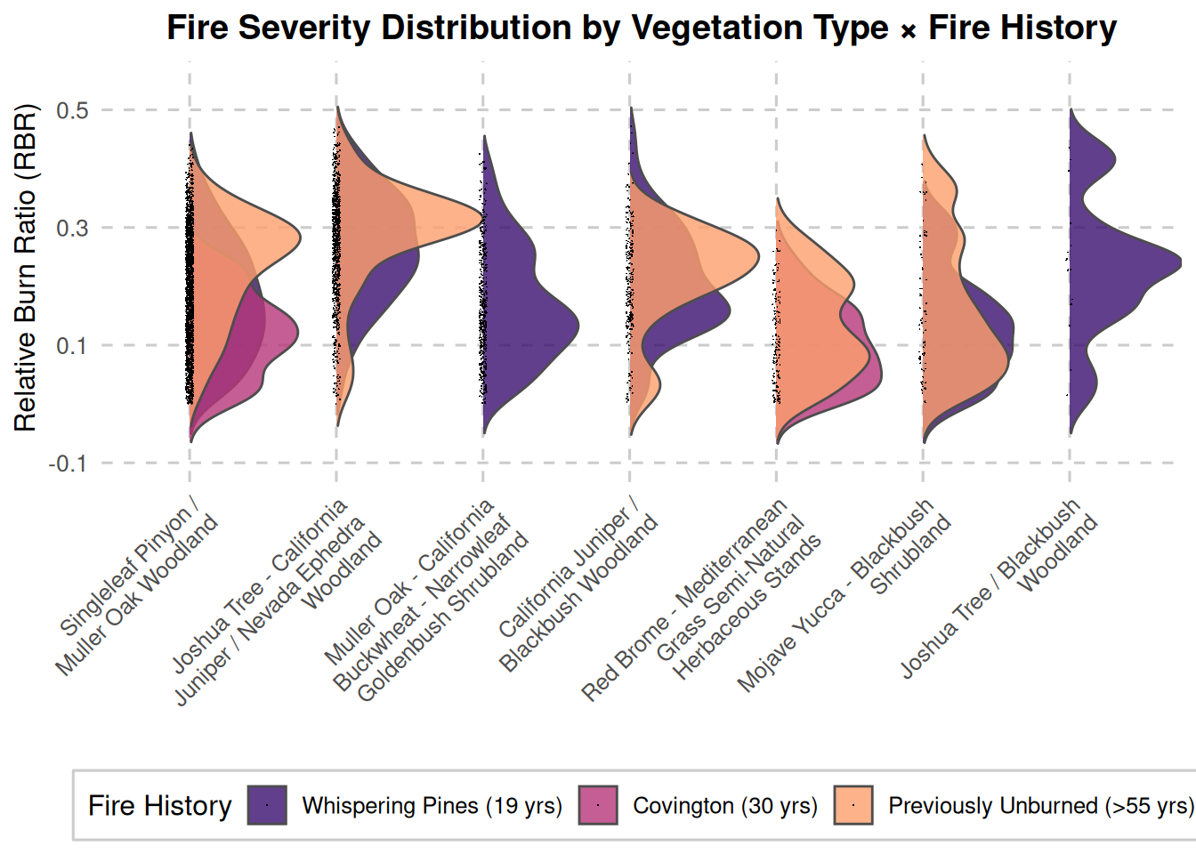
#remove 'association' from unit names
ordered_veg_clean <- ordered_veg %>%
  str_remove_all("Association") %>%
  str_squish()

all_vals_ordered <- all_vals %>% 
  mutate(MapUnit_Name = str_squish(str_remove_all(MapUnit_Name, "Association")), MapUnit_Name = factor(MapUnit_Name, levels = ordered_veg_clean, ordered = TRUE))

# build legend labels
legend_labs <- c("WHISPERING PINES" = sprintf("Whispering Pines (19 yrs)"),
                 "COVINGTON" = sprintf("Covington (30 yrs)"),
                 "Previously Unburned" = "Previously Unburned (>55 yrs)")

ggplot(all_vals_ordered, aes(x= value, y = MapUnit_Name, fill = FIRE_NAME)) +
  geom_density_ridges(scale = 1.0, rel_min_height  = 0.01, trim = FALSE, 
                      colour = "grey30", alpha = 0.8, size = 0.2) +
  geom_jitter(aes(x = value, y = MapUnit_Name), height = 0.025, 
             size = .5, stroke = 0, shape = 20) +
  coord_flip() +
  scale_x_continuous(name = " Relative Burn Ratio (RBR)", 
                     breaks = seq(-0.1, 0.6, by = 0.2), limits = c(-0.1, 0.55)) +
  scale_y_discrete(name = NULL, labels = function(x) str_wrap(x, 25)) +
  scale_fill_viridis_d(name = "Fire History", option  = "magma", begin = 0.2, 
                       end = 0.8, labels = legend_labs) +
  labs(title = "Fire Severity Distribution by Vegetation Type × Fire History") +
  theme_minimal(base_size = 12) +
  theme(axis.text.x  = element_text(angle = 45, hjust = 1),
        axis.text.y = element_text(size = 10),
        panel.grid.major = element_line(color = "grey80", linetype = "dashed"),
        panel.grid.minor = element_blank(),
        plot.title = element_text(face = "bold", hjust = 0.5),
        legend.position = "bottom",
        legend.background = element_rect(fill = "white", color = "grey80"))