Black Rock Fire Exploration

Published

October 27, 2025

Setup

Load required libraries

library(tidyverse)        
library(sf)            
library(raster)          
library(exactextractr)    
library(leaflet)         
library(htmlwidgets)     
library(viridis)        
library(readr)
library(scales)
library(ggridges)
library(RColorBrewer)

Read data

veg_data <- st_read(dsn = "../../shared_inputs/jotrgeodata.gpkg",layer = "JOTR_VegPolys", 
                    quiet = TRUE)

# Read fire severity (raster)
rbr_rast <- raster("inputs/refined_rbr.tif")

Interactive map of fire location

# Build two palette functions (to force descending order in leaflet legend) :
pal      <- colorNumeric("plasma", domain = values(rbr_rast), 
                         na.color = "transparent")
pal_rev  <- colorNumeric("plasma", domain = values(rbr_rast), 
                         na.color = "transparent", reverse = TRUE)

# Draw the map
leaflet(options = leafletOptions(attributionControl = TRUE)) %>%
  addProviderTiles("CartoDB.Positron") %>% # Use the reversed palette for the raster itself
  addRasterImage(rbr_rast, colors = pal_rev, opacity = 0.6,project = FALSE) %>% # Use the normal palette + label transform for the legend
  addLegend(position= "bottomright", pal = pal, values = values(rbr_rast), 
            title = "RBR value",
            labFormat = labelFormat(transform = function(x) sort(x, decreasing = TRUE)))

Static RBR map with grid

# Turn the RasterLayer into a data.frame
rbr_df <- as.data.frame(rasterToPoints(rbr_rast))
colnames(rbr_df) <- c("x", "y", "RBR")

ggplot(rbr_df, aes(x = x, y = y, fill = RBR)) +
  geom_raster() +
  scale_fill_viridis_c(option = "plasma", direction = -1,  na.value  = "transparent",
    name = "RBR value") +
  coord_equal() +
  labs(title = "Refined Relative Burn Ratio (RBR)", x = NULL, y = NULL) +
  theme_minimal(base_size = 12) +
  theme(panel.grid.major = element_blank(),
        panel.grid.minor = element_blank(),
        panel.border = element_rect(fill = NA, color = "black", size = 0.5),
        axis.ticks = element_line(color = "black"),
        axis.text = element_text(color = "black"),
        panel.background = element_blank(),
        legend.position = "right")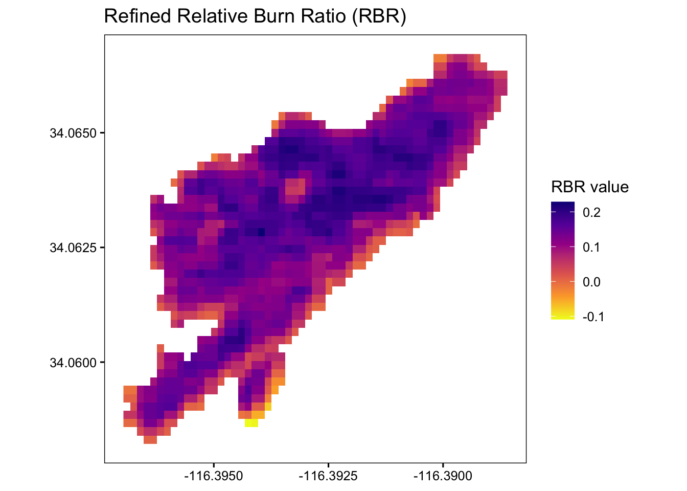

Reproject raster to match vegetation data and calculate area

For the purpose of this analysis, we reprojected the fire severity raster into NAD83 / UTM zone 11N to match the vegetation map, which may introduce some imprecision of sentinel 2 cells

# Grab the vector’s CRS as a PROJ4/WKT string
vec_crs <- st_crs(veg_data)$proj4string

# Reproject the raster to that CRS
#    - use method="bilinear" for continuous data
rbr_to_vec_crs <- projectRaster(rbr_rast, crs = vec_crs, method = "bilinear")

Extract fire perimeter from raster

# Polygonize all positive, non‐NA cells from the reprojected raster, convert to sf und merge into a single boundary polygon
fire_boundary <- rasterToPolygons(rbr_to_vec_crs, fun = function(x) !is.na(x) & x > 0, 
                          dissolve = TRUE) %>%
  st_as_sf() %>%
  st_union() 

# Write to file
if (file.exists("outputs/fire_perimeter/severity_to_fire_perimeter.shp")) {
  file.remove("outputs/fire_perimeter/severity_to_fire_perimeter.shp")
}

[1] TRUE

st_write(fire_boundary, "outputs/fire_perimeter/severity_to_fire_perimeter.shp")

Writing layer `severity_to_fire_perimeter' to data source 
  `outputs/fire_perimeter/severity_to_fire_perimeter.shp' using driver `ESRI Shapefile'
Writing 1 features with 0 fields and geometry type Polygon.

#convert reprojected raster to dataframe
rbr_to_vec_crs_df <- as.data.frame(rasterToPoints(rbr_to_vec_crs))
colnames(rbr_to_vec_crs_df) <- c("x", "y", "RBR")

#plot fire severity with generated fire boundary 
ggplot() +
  geom_raster(data = rbr_to_vec_crs_df, aes(x = x, y = y, fill = RBR)) +
  geom_sf(data = fire_boundary, fill = NA, color = "black", linewidth = 0.8) +
  scale_fill_viridis_c(option = "plasma", direction = -1,  na.value  = "transparent",
    name = "RBR value") +
  coord_sf() +
  labs(title = "Burned Area Boundary (RBR > 0)", x = NULL, y = NULL) +
  theme_minimal(base_size = 12) +
  theme(panel.grid.major = element_blank(),
        panel.grid.minor = element_blank(),
        panel.border = element_rect(fill = NA, color = "black", size = 0.5),
        axis.ticks = element_line(color = "black"),
        axis.text = element_text(color = "black"),
        axis.text.x = element_text(angle = 45, hjust = 1),
        panel.background = element_blank(),
        legend.position = "right")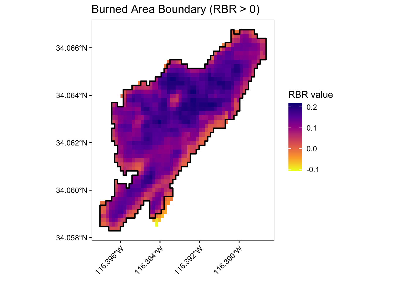

Clip vegetation data to fire boundary and ummarize vegetation types within fire boundary

# Ensure CRS metadata match before intersection (sf requires exact equality)
if (!identical(st_crs(veg_data), st_crs(fire_boundary))) {
  st_crs(fire_boundary) <- st_crs(veg_data)
}

# Calculate area per vegetation type polygon
clipped_veg <- st_intersection(veg_data, fire_boundary) %>%
  mutate(area_ha = as.numeric(st_area(.) / 10000))  # m² → ha

# Summarize hectares by vegetation type
veg_summary <- clipped_veg %>%
  st_set_geometry(NULL) %>%          # drop geometry for speed
  group_by(MapUnit_Name) %>%
  summarise(veg_ha = sum(area_ha, na.rm = TRUE), .groups = "drop") %>%
  mutate(pct_of_total = 100 * veg_ha / sum(veg_ha)) %>%# total area can be calculated in pipe
  bind_rows(tibble(MapUnit_Name = "Total Burned Area", 
                   veg_ha = sum(clipped_veg$area_ha), pct_of_total = 100)) %>%
  arrange(desc(pct_of_total))

# write out
write_csv(veg_summary, "outputs/veg_burned_summary.csv")

# show table
knitr::kable(veg_summary)

MapUnit_Name	veg_ha	pct_of_total
Total Burned Area	32.0688000	100.000000
California Juniper / Blackbush Woodland Association	11.9089824	37.135728
Joshua Tree - California Juniper / Nevada Ephedra Woodland Association	9.2589004	28.871989
California Juniper / Muller Oak - Blackbush Woodland Association	5.1757861	16.139631
Singleleaf Pinyon / Muller Oak Woodland Association	3.2751304	10.212825
Catclaw Acacia - Desert Almond Shrubland Association	1.1892117	3.708314
Catclaw Acacia - (Sweetbush - Desert Lavender) Shrubland Association	0.7169604	2.235695
Joshua Tree / Blackbush Woodland Association	0.5438286	1.695818

Assertions

# After creating fire_boundary
fire_boundary_area <- st_area(fire_boundary) %>% units::set_units("ha")
cat("Total fire boundary area (ha):", fire_boundary_area, "\n")

Total fire boundary area (ha): 32.0688

# After clipping vegetation
total_veg_area <- sum(clipped_veg$area_ha)
cat("Sum of vegetation areas within fire (ha):", total_veg_area, "\n")

Sum of vegetation areas within fire (ha): 32.0688

# Assert that these are approximately equal (within small tolerance for computational differences)
stopifnot(abs(as.numeric(fire_boundary_area) - total_veg_area) < 0.1)

Map vegetation types and their area within fire boundary

# Join summary back to clipped polygons
clipped_joined <- clipped_veg %>%
    dplyr::left_join(dplyr::select(veg_summary, MapUnit_Name, veg_ha, pct_of_total),
    by = "MapUnit_Name")

# Create an ordered factor of vegetation types
ordered_types <- veg_summary %>%
  filter(MapUnit_Name != "Total Burned Area") %>%
  arrange(desc(pct_of_total)) %>%
  pull(MapUnit_Name)

# Pick colors from the Set3 palette
n_types   <- length(ordered_types)
set3_cols <- brewer.pal(n = max(3, n_types), "Set3")[1:n_types]
names(set3_cols) <- ordered_types

# Build legend labels without the word “Association”
legend_labels <- veg_summary %>%
  filter(MapUnit_Name != "Total Burned Area") %>%
  mutate(clean_name = MapUnit_Name %>% # remove “Association” and clean up whitespace
           str_remove_all("Association") %>%
           str_squish(),
         label = sprintf("%s\n%.1f ha (%.1f%%)",
                         clean_name,
                         veg_ha,
                         pct_of_total)) %>%
  pull(label) %>%
  set_names(ordered_types)  # keep the same factor levels for mapping

# Total burned area for caption
total_fire_ha <- veg_summary %>%
  filter(MapUnit_Name == "Total Burned Area") %>%
  pull(veg_ha)

# wrap your legend labels to ~30 chars per line
legend_labels_wrapped <- legend_labels %>% 
  lapply(str_wrap, width = 30) %>% 
  unlist(use.names = TRUE)

#plot
ggplot(clipped_joined) +
  geom_sf(aes(fill = factor(MapUnit_Name, levels = ordered_types)),
          color = "gray80", size = 0.2) +
  scale_fill_manual(values = set3_cols, labels = legend_labels_wrapped, 
                    name   = "Vegetation Type:\nArea (ha) & % of Total") +
  coord_sf(crs = st_crs(4326)) +   # keep geographic graticule if you like
  labs(title   = "", caption = sprintf("Total Burned Area: %.1f ha", total_fire_ha)) +
  theme_minimal(base_size = 10) +
  theme(panel.grid.major = element_blank(),
        panel.grid.minor = element_blank(),
        panel.border = element_rect(fill = NA, color = "black", size = 0.5),
        panel.background = element_blank(),
        axis.text.x = element_text(angle = 45, hjust = 1),  # ← slanted labels
        axis.text.y = element_text(size = 8),
        axis.ticks = element_line(color = "black"),
        axis.title = element_blank(),
        legend.position = "right",
        legend.text = element_text(size = 9),
        legend.title = element_text(size = 10, face = "bold"),
        legend.key.height = unit(1, "cm"),     # ↑ match the guide keyheight
        legend.spacing.y = unit(1, "cm"), 
        plot.caption = element_text(hjust  = 2.5, margin = margin(b = 2)))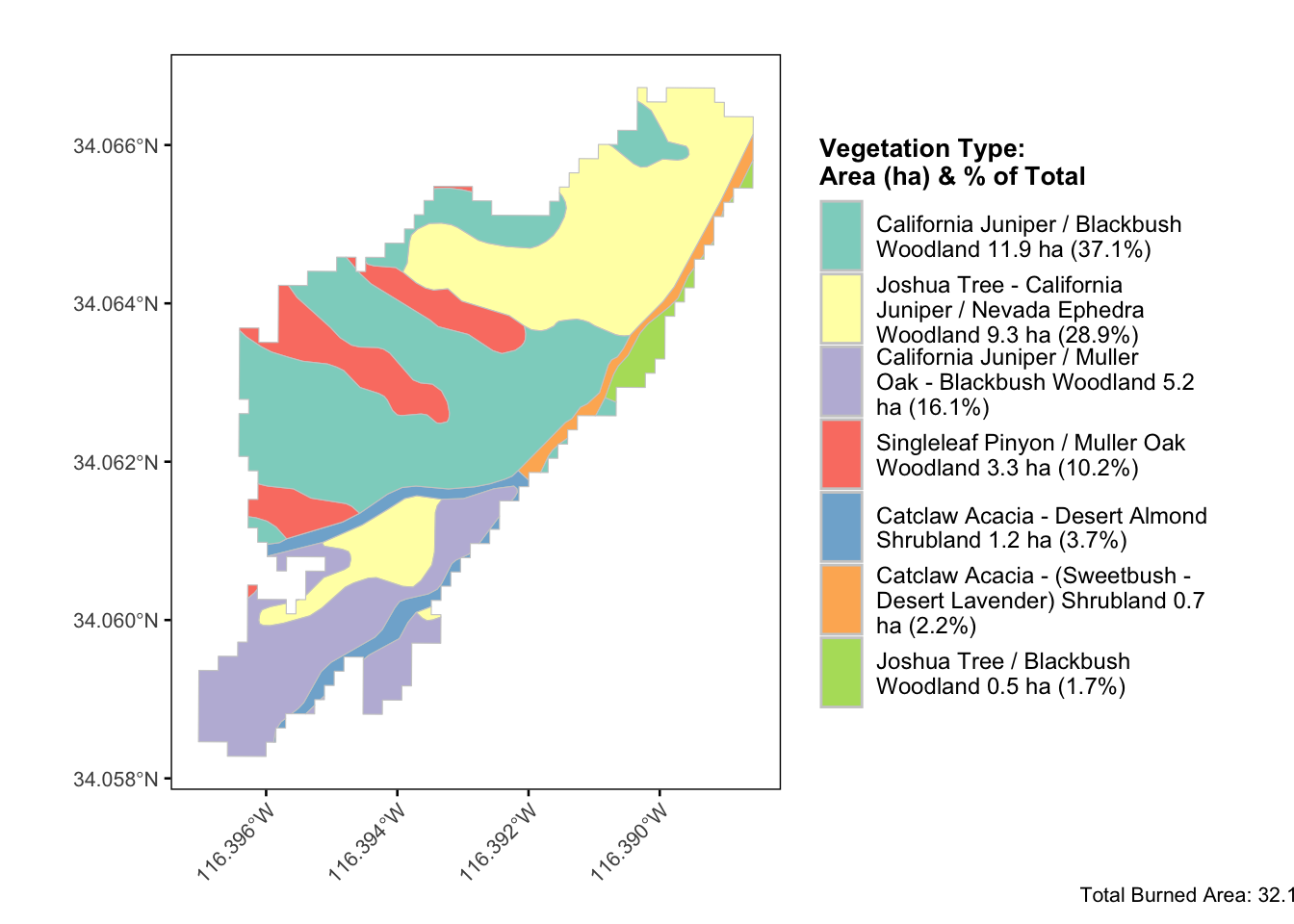

Summary statistics of fire severity by vegetation type

merged_units_veg <- clipped_veg %>%
  dplyr::select(MapUnit_Name, SHAPE) %>% 
  group_by(MapUnit_Name) %>%
  summarise(do_union = TRUE, .groups = "drop")

 # Compute per-polygon stats
clipped_stats <- merged_units_veg %>%
  mutate(min_RBR = exact_extract(rbr_to_vec_crs, ., "min",progress = FALSE),
         max_RBR = exact_extract(rbr_to_vec_crs, ., "max",progress = FALSE),
         mean_RBR = exact_extract(rbr_to_vec_crs, ., "mean",progress = FALSE),
         median_RBR = exact_extract(rbr_to_vec_crs, ., "median",progress = FALSE),
         sd_RBR = exact_extract(rbr_to_vec_crs, ., "stdev",progress = FALSE),
         n_pixels = exact_extract(rbr_to_vec_crs, ., "count",progress = FALSE))


#  Reorder to your preferred sequence
ordered_veg <- c("California Juniper / Blackbush Woodland Association",
                 "Joshua Tree - California Juniper / Nevada Ephedra Woodland Association",
                 "California Juniper / Muller Oak - Blackbush Woodland Association",
                 "Singleleaf Pinyon / Muller Oak Woodland Association",
                 "Catclaw Acacia - Desert Almond Shrubland Association",
                 "Catclaw Acacia - (Sweetbush - Desert Lavender) Shrubland Association",
                 "Joshua Tree / Blackbush Woodland Association")

severity_summary <- clipped_stats %>%
  slice(match(ordered_veg, MapUnit_Name))  %>%
  st_set_geometry(NULL)


#Write
write_csv(severity_summary, "outputs/severity_veg_summary.csv")

# View results
knitr::kable(
  severity_summary)

MapUnit_Name	min_RBR	max_RBR	mean_RBR	median_RBR	sd_RBR	n_pixels
California Juniper / Blackbush Woodland Association	-0.0212007	0.2120353	0.1292027	0.1340394	0.0445410	437.83023
Joshua Tree - California Juniper / Nevada Ephedra Woodland Association	-0.0109042	0.2145325	0.1431141	0.1513706	0.0434168	340.40076
California Juniper / Muller Oak - Blackbush Woodland Association	-0.0376531	0.2011088	0.0885313	0.0883403	0.0506465	190.28625
Singleleaf Pinyon / Muller Oak Woodland Association	0.0127173	0.2167048	0.1330115	0.1396981	0.0476073	120.40921
Catclaw Acacia - Desert Almond Shrubland Association	0.0006624	0.1616597	0.0663210	0.0601768	0.0413764	43.72102
Catclaw Acacia - (Sweetbush - Desert Lavender) Shrubland Association	0.0003514	0.1679855	0.0480873	0.0433495	0.0364539	26.35884
Joshua Tree / Blackbush Woodland Association	-0.0030923	0.1362080	0.0559410	0.0429493	0.0335164	19.99370

Plot fire severity by vegetation type

# Extract pixel values per polygon directly
vals_list <- extract(rbr_to_vec_crs, merged_units_veg)

# Build long tibble
vals_df <- tibble(MapUnit_Name = merged_units_veg$MapUnit_Name, value = vals_list) %>%
  unnest(cols = c(value)) %>%
  filter(!is.na(value)) %>%
  mutate(MapUnit_Name = factor(MapUnit_Name, levels = ordered_veg))

# Prepare colors & wrapped labels
set3_cols      <- brewer.pal(length(ordered_veg), "Set3")
names(set3_cols) <- ordered_veg
labels_wrapped <- str_wrap(ordered_veg, width = 25)

#  Plot
ggplot(vals_df, aes(x = MapUnit_Name, y = value, fill = MapUnit_Name)) +
  geom_violin(trim = FALSE, color = "black", alpha = 0.8) +
  stat_summary(fun = median, geom = "point", size = 1.5, color = "black") +
  scale_fill_manual(values = set3_cols, guide = FALSE) +
  scale_x_discrete(labels = labels_wrapped) +
  labs(x = NULL,
       y = "Refined Relative Burn Ratio (RBR)",
       title = "Fire Severity Distribution by Vegetation Type\n(ordered left → right by % burned area)") +
  theme_minimal(base_size = 12) +
  theme(axis.text.x = element_text(angle = 45, hjust = 1, size = 10),
        panel.grid.major.y = element_line(color = "grey80", linetype = "dashed"),
        panel.grid.major.x = element_blank(),
        panel.grid.minor = element_blank(),
        plot.title = element_text(hjust = 0.5, size = 14))

Load Historical Fires

# Read the historic‐fires shapefile
fire_hist <- st_read("../../shared_inputs/HistFires_JOTR_MOJA/FindExistingLocationsOutput.shp") %>% # Reproject into EPSG:26911 (NAD83 / UTM zone 11N)
  st_transform(26911)

Map historical fires and Black Rock fire boundary

#  palette for all years —
fire_years <- sort(unique(fire_hist$YEAR_))
pal_fire <- setNames(viridis(n = length(fire_years), option = "turbo"), fire_years)

# create a 100% buffer around the Black Rock fire polygon
#    (buffer distance = max(width, height) of its bbox)
fb <- fire_boundary %>%
  st_union() %>% # ensure single geometry
  {
    bb  <- st_bbox(.)
    dist <- max(bb$xmax - bb$xmin, bb$ymax - bb$ymin)
    st_buffer(., dist) 
  }

# find which historic fires intersect that buffer
visible_yr <- fire_hist %>%
  filter(st_intersects(., fb, sparse = FALSE)) %>%
  pull(YEAR_) %>%
  unique() %>%
  sort()

# plot
ggplot() +
  geom_sf(data = fire_hist, aes(fill = factor(YEAR_)), colour = "black", 
          size = 0.2, alpha = 0.6) +
  geom_sf(data = fire_boundary, fill   = NA, colour = "red", size = 1) +
  coord_sf(xlim = st_bbox(fb)[c("xmin", "xmax")], ylim = st_bbox(fb)[c("ymin", "ymax")],
           expand = FALSE) +
  scale_fill_manual(name   = "Fire Year", values = pal_fire, breaks = visible_yr) +
  labs(title = "Historical Fires & Black Rock Fire Boundary") +
  theme_void(base_size = 14) +
  theme(legend.position = c(0.85, 0.85),
        legend.background = element_rect(fill = "white", color = "grey80"),
        legend.title = element_text(face = "bold", size = 10),
        legend.text = element_text(size = 8),
        plot.title = element_text(hjust = 0.5, size = 16))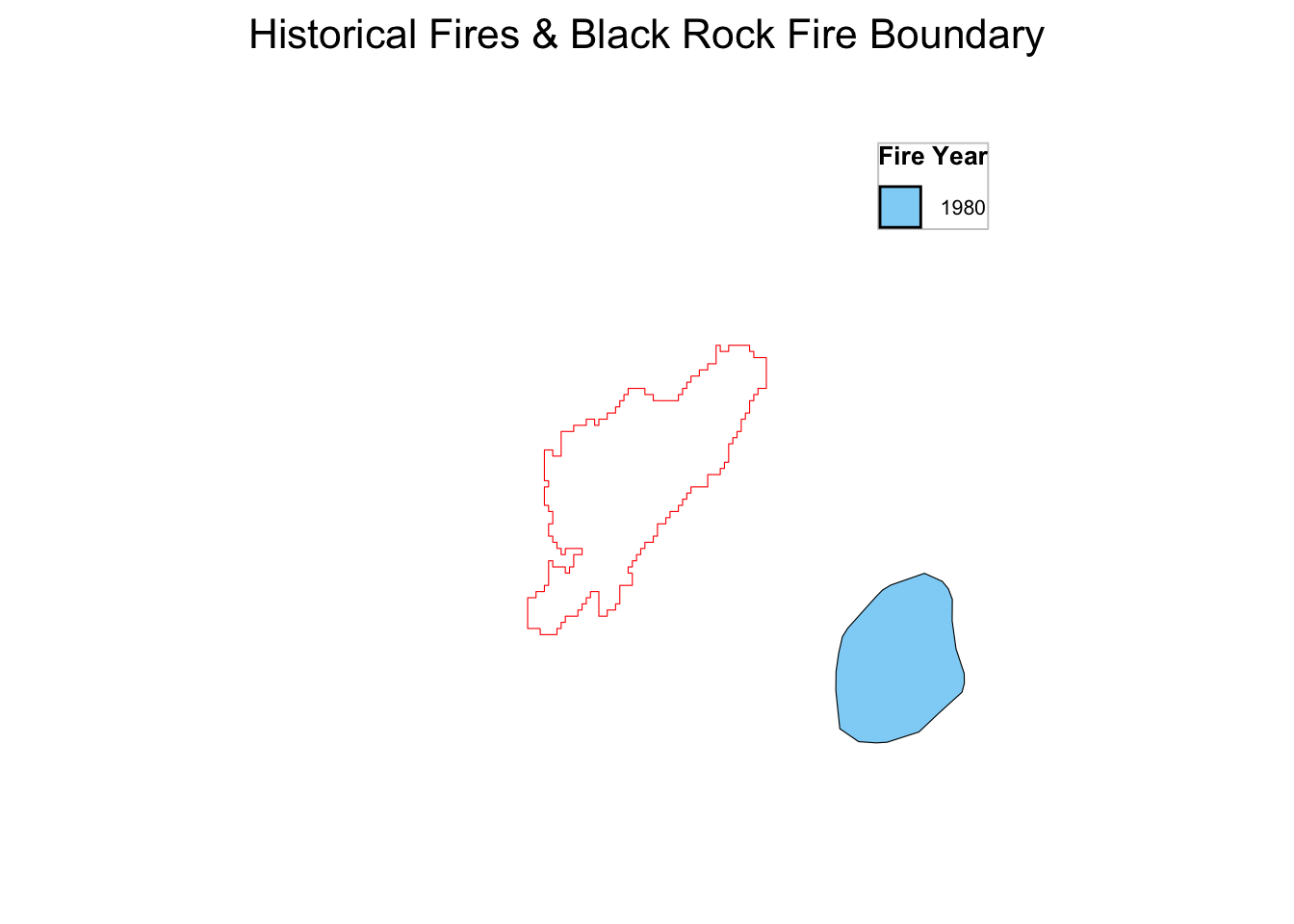

Summary statistics of fire severity by historical fire

#  Intersection of historic fires & Black Rock boundary
burned_overlap <- st_intersection(fire_hist, fire_boundary)

# Burned stats by YEAR_ + FIRE_NAME (still sf)
burned_stats <- burned_overlap %>%
  mutate(min_RBR = exact_extract(rbr_to_vec_crs, ., "min",progress = FALSE),
         max_RBR = exact_extract(rbr_to_vec_crs, ., "max",progress = FALSE),
         mean_RBR = exact_extract(rbr_to_vec_crs, ., "mean",progress = FALSE),
         sd_RBR = exact_extract(rbr_to_vec_crs, ., "stdev",progress = FALSE),
         area_ha = st_area(geometry)/10000) %>%
  dplyr::select(FIRE_NAME, YEAR_, min_RBR, max_RBR, mean_RBR, sd_RBR, area_ha)


#  Unburned remainder stats (also an sf)
unburned_stats <- st_sf(FIRE_NAME = "Previously Unburned", YEAR_ = 0,
                        geometry  = st_sfc(st_difference(st_union(fire_boundary), st_union(burned_overlap))),
    crs       = st_crs(fire_boundary)) %>%
  mutate(min_RBR = exact_extract(rbr_to_vec_crs, ., "min",progress = FALSE),
         max_RBR = exact_extract(rbr_to_vec_crs, ., "max",progress = FALSE),
         mean_RBR = exact_extract(rbr_to_vec_crs, ., "mean",progress = FALSE),
         sd_RBR = exact_extract(rbr_to_vec_crs, ., "stdev",progress = FALSE),
         area_ha = st_area(geometry)/10000) %>%
  dplyr::select(FIRE_NAME, YEAR_, min_RBR, max_RBR, mean_RBR, sd_RBR, area_ha)


#  Combine
full_fire_history <- bind_rows(burned_stats, unburned_stats)

# Plot:
# plot(full_fire_history["FIRE_NAME"])

# Drop geometry and fix the NA‐row
full_fire_history_table <- full_fire_history %>%
  st_set_geometry(NULL) %>%
  mutate(YEAR_  = if_else(is.na(YEAR_), 0L, YEAR_),
         FIRE_NAME = if_else(is.na(FIRE_NAME), "Unburned", FIRE_NAME))


#Write
write_csv(full_fire_history_table, "outputs/severity_fire_history.csv")

# Display
knitr::kable(
  full_fire_history_table)

FIRE_NAME	YEAR_	min_RBR	max_RBR	mean_RBR	sd_RBR	area_ha
Previously Unburned	0	-0.0352443	0.2167048	0.1216562	0.0518731	32.0688 [m^2]

Assertions

burned_area_sum <- sum(as.numeric(st_area(burned_overlap))) / 10000
unburned_area <- as.numeric(st_area(unburned_stats)) / 10000
total_calculated_area <- burned_area_sum + unburned_area

cat("Sum of historical burned areas (ha):", burned_area_sum, "\n")

Sum of historical burned areas (ha): 0

cat("Unburned area (ha):", unburned_area, "\n")

Unburned area (ha): 32.0688

cat("Total calculated area (ha):", total_calculated_area, "\n")

Total calculated area (ha): 32.0688

cat("Total fire boundary area (ha):", as.numeric(fire_boundary_area), "\n")

Total fire boundary area (ha): 32.0688

# Check these are approximately equal
stopifnot(abs(total_calculated_area - as.numeric(fire_boundary_area)) < 0.1)